Factorized Explainer for Graph Neural Networks
Rundong Huang1, Farhad Shirani2*, Dongsheng Luo2*
1Technical University of Munich, Munich, Germany
2Florida International University, Miami, U.S.
rundong.huang@tum.de,
{fshirani,dluo
}@fiu.edu
Abstract
Graph Neural Networks (GNNs) have received increasing
attention due to their ability to learn from graph-structured
data. To open the black-box of these deep learning models,
post-hoc instance-level explanation methods have been
proposed to understand GNN predictions. These methods
seek to discover substructures that explain the prediction
behavior of a trained GNN. In this paper, we show
analytically that for a large class of explanation tasks,
conventional approaches, which are based on the principle of
graph information bottleneck (GIB), admit trivial solutions
that do not align with the notion of explainability. Instead, we
argue that a modified GIB principle may be used to avoid the
aforementioned trivial solutions. We further introduce a novel
factorized explanation model with theoretical performance
guarantees. The modified GIB is used to analyze the
structural properties of the proposed factorized explainer.
We conduct extensive experiments on both synthetic and
real-world datasets to validate the effectiveness of our
proposed factorized explainer.
Introduction
Graph-structured data is ubiquitous in real-world applications,
manifesting in various domains such as social networks (Fan
et al. 2019), molecular structures (Mansimov et al. 2019; Chereda
et al. 2019), and knowledge graphs (Liu et al. 2022). This has
led to significant interest in learning methodologies specific to
graphical data, particularly, graph neural networks (GNNs).
GNNs commonly employ message-passing mechanisms,
recursively transmitting and fusing messages among neighboring
nodes on graphs. Thus, the learned node representation
captures both node attributes and neighborhood information,
thereby enabling diverse downstream tasks such as node
classification (Kipf and Welling 2017; Veličković et al. 2018),
graph classification (Xu et al. 2019), and link prediction (Lu et al. 2022).
Despite the success of GNNs in a wide range of domains, their
inherent “black-box” nature and lack of interpretability, a
characteristic shared among many contemporary machine
learning methods, is a major roadblock in their utility in sensitive
application scenarios such as autonomous decision systems.
To address this, various GNN explanation methods have
been proposed to understand the graph-structured data and
associated deep graph learning models (Ying et al. 2019; Luo
et al. 2020; Yuan et al. 2022). In particular, post-hoc
instance-level explanation methods provide an effective way
to identify determinant substructures in the input graph,
which plays a vital role in trustworthy deployments (Ying
et al. 2019; Luo et al. 2020). In the context of graph
classification, the objective of graph explanation methods is,
given a graph G, to extract a minimal and sufficient subgraph,
G*, that can be used to determine the instance label, Y .
The Graph Information Bottleneck principle (GIB) (Wu
et al. 2020) provides an intuitive principle that is widely
adopted as a practical instantiation. At a high level, the GIB
principle finds the subgraph G* which minimizes the mutual
information between the original graph G and the subgraph G*
and maximizes the mutual information between the subgraph G*
and instance label Y by minimizing I(G,G*) - αI(G*,Y ),
where the hyperparameter α > 0 captures the tradeoff between
minimality and informativeness of G* (Miao, Liu, and
Li 2022). As an example, the GNNExplainer method operates
by finding a learnable edge mask matrix, which is optimized by
the GIB objective (Ying et al. 2019). The PGExplainer also
uses a GIB-based objective and incorporates a parametric
generator to learn explanatory subgraphs from the model’s
output (Luo et al. 2020).
There are several limitations in the existing explainability
approaches. First, as shown analytically in this work, existing
GIB-based methods suffer from perceptually unrealistic
explanations. Specifically, we show that in a wide-range of
statistical scenarios, the original GIB formulation of the
explainability problem has a trivial solution where the achieved
explanation G*signals the predicted value of Y , but is independent
of the input graph G, otherwise. That is, the Markov chain
G*↔ Y ↔ G holds. As a result, the explanation G* optimizing
the GIB objective may consist of a few disconnected edges and
fails to align with the high-level notion of explainability. To
alleviate this problem, PGExplainer includes an ad-hoc
connectivity constraint as the regularization term (Luo
et al. 2020). However, without theoretical guarantees,
the effectiveness of the extra regularization is marginal in
more complicated datasets (Shan et al. 2021). Second,
although previous parametric explanation methods, such
as PGExplainer (Luo et al. 2020) and ReFine (Wang
et al. 2021), are efficient in the inductive setting, these methods
neglect the existence of multiple motifs, which is routinely
observed in real-life datasets. For example, In the MUTAG
dataset (Debnath et al. 1991), both chemical components
NO2 and NH2, which can be considered as explanation
subgraphs, contribute to the positive mutagenicity. Existing
methods over-simplify the relationship between motifs
and labels to one-to-one, leading to inaccuracy in real-life
applications.
To address these issues, we first analytically investigate the
pitfalls of the application of the GIB principle in explanation
tasks from an information theoretic perspective, and propose
a modified GIB principle that avoids these issues. To
further improve the inductive performance, we propose a
new framework to unify existing parametric methods and
show that their suboptimality is caused by their locality
property and the lossy aggregation step in GNNs. We further
propose a straightforward and effective factorization-based
explanation method to break the limitation of existing local
explanation functions. We summarize our main contributions as
follows.
-
For the first time, we point out that the gap between
the practical objective function (GIB) and high-level
objective is non-negligible in the most popular post-hoc
explanation framework for graph neural networks.
-
We derive
a generalized framework to unify existing parametric
explanation methods and theoretically analyze their
pitfalls in achieving accurate explanations in complicated
real-life datasets. We further propose a straightforward
explanation method with a solid theoretical foundation to
achieve better generalization capacity.
-
Comprehensive empirical studies on both synthetic
and real-life datasets demonstrate that our method can
consistently improve the quality of the explanations.
Preliminary
Notations and Problem Definition
A graph G is parameterized by a quadruple
( ,
, ;Z,A), where i) = {v1,v2,...,vn} is the
node/vertex
set, ii) ⊆× is the edge set, iii) Z ∈ℝn×d is the feature
matrix, where the ith row of Z, denoted by zi ∈ℝ1×d, is the
d-dimensional feature vector associated with node vi,i ∈ [n],
and iv) the adjacency matrix A ∈{0,1}n×n is determined by
the edge set , where Aij = 1 if (vi,vj) ∈, Aij = 0,
otherwise. We write |G| and || interchangeably to denote the
number of edges of G.
;Z,A), where i) = {v1,v2,...,vn} is the
node/vertex
set, ii) ⊆× is the edge set, iii) Z ∈ℝn×d is the feature
matrix, where the ith row of Z, denoted by zi ∈ℝ1×d, is the
d-dimensional feature vector associated with node vi,i ∈ [n],
and iv) the adjacency matrix A ∈{0,1}n×n is determined by
the edge set , where Aij = 1 if (vi,vj) ∈, Aij = 0,
otherwise. We write |G| and || interchangeably to denote the
number of edges of G.
For graph classification task, each graph Gi has a label
Y i ∈ , with a GNN model f trained to classify Gi into its class,
i.e., f : G
, with a GNN model f trained to classify Gi into its class,
i.e., f : G {1,2,
{1,2, ,||}. For the node classification task,
each graph Gi denotes a K-hop sub-graph centered around node
vi, with a GNN model f trained to predict the label for node
vi based on the node representation of vi learned from
Gi.
,||}. For the node classification task,
each graph Gi denotes a K-hop sub-graph centered around node
vi, with a GNN model f trained to predict the label for node
vi based on the node representation of vi learned from
Gi.
Informative feature selection has been well studied in non-graph
structured data (Li et al. 2017), and traditional methods, such
as concrete autoencoder (Abid, Balin, and Zou 2019),
can be directly extended to explain features in GNNs. In
this paper, we focus on discovering important typologies.
Formally, the obtained explanation G* is characterized by a
binary mask M ∈{0,1}n×n on the adjacency matrix,
e.g., G* = (,,A ⊙M;Z), where ⊙ is elements-wise
multiplication. The mask highlights components of G which
influence the output of f.
Graph Information Bottleneck
The GIB principle refers to the graphical version of the
Information Bottleneck (IB) principle (Tishby and
Zaslavsky 2015) which offers an intuitive measure for
learning dense representations. It is based on the notion
that an optimal representation should contain minimal and
sufficient information for the downstream prediction task.
Recently, a high-level unification of several existing post hoc
GNN explanation methods, such as GNNExplainer (Ying
et al. 2019), and PGExplainer (Luo et al. 2020) was
provided using this concept (Wu et al. 2020; Miao, Liu, and
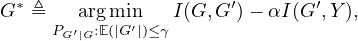
Li 2022; Yu et al. 2021). Formally, prior works have
represented the objective of finding an explanation graph G* in
G as follows:
where G* is the explanation subgraph, γ ∈ℕ is the maximum
expected size (number of edges) of the explanation, Y is the
original or ground truth label, and α is a hyper-parameter
capturing the trade-off between minimality and sufficiency
constraints. At a high level, the GIB formulation given in
equation 1 selects the minimal explanation G′, by minimizing
I(G,G′) and imposing E(|G′|) ≤ γ, that inherits only the most
indicative information from G to predict the label Y , by
maximizing I(G′,Y ), while avoiding imposing potentially
biased constraints, such the connectivity of the selected
subgraphs and exact maximum size constraints (Miao,
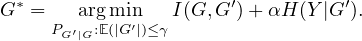
Liu, and Li 2022). Note that from the definition of mutual
information, we have I(G′,Y ) = H(Y ) -H(Y |G′), where the
entropy H(Y ) is static and independent of the explanation
process. Thus, minimizing the mutual information between the
explanation subgraph G′ and Y can be reformulated as
maximizing the conditional entropy of Y given G′. That
is:
Graph Information Bottleneck for Explanation
In this section, we study several pitfalls arising from the
application of the GIB principle to explanation tasks. We
demonstrate that, for a broad range of learning tasks, the original
GIB formulation of the explainability problem has a trivial solution that does not align with the intuitive notion of
explainability. We propose a modified version of the GIB
principle that avoids this trivial solution and is applicable in
constructing GNN explanation methods. The analytical
derivations in subsequent sections will focus on this modified
GIB principle. To elaborate, we argue that the optimization
given in equation 2 is prone to signaling issues and, in
general, does not fully align theoretically with the notion of
explainability. More precisely, the GIB formulation allows for
an explanation algorithm to output G* which signals the
predicted value of Y , but is independent of the input graph G
otherwise. To state this more concretely, we consider the class of
statistically degraded classification tasks defined in the
following.
Remark 1. Any deterministic classification task, where
there exists a function h :  →
→ such that h(X) = Y , is
statistically degraded.
such that h(X) = Y , is
statistically degraded.
Remark 2. There are classification tasks that are not
statistically degraded. For instance, let us consider a
classification task in which the feature vector is X =
(X1,X2), where X1 and X2 are independent binary
symmetric variables. Let the label Y be equal to X1 with
probability p ∈ (0,1) and equal to X2, otherwise. By
exhaustively searching over all 16 possible choices of h(X),
it can be verified that no Boolean function h(X) exists
such that the relationship X ↔ h(X) ↔ Y holds.
Consequently, the classification task (,,PX,Y ) is not
statistically degraded.
Remark 3. Note that for the statistically degraded task
defined in Definition 1, the optimal classifier f*(X) is equal
to the sufficient statistic h(X).
In order to show the limitations of the GIB in fully encapsulating
the concept of explainability, in the sequel we focus on
statistically degraded classification tasks involving graph inputs.
That is, we take X = G, where G is the input graph. The next
lemma shows that, for any statistically degraded task, there
exists an explanation function Ψ(⋅) which optimizes the
GIB objective function (equation 2), and whose output is
independent of G given h(⋅). That is, although the explanation
algorithm is optimal in the GIB sense, it does not provide any
additional information about the input of the classifier, in
addition to the information that the classifier output label h(G)
readily provides.
Theorem 1. Consider a statistically degraded graph
classification task, parametrized by (PG,Y ,h(⋅)), where
PG,Y is the joint distribution of input graphs and their
labels, and h :  →is such that G ↔ h(G) ↔ Y holds.
For any α > 0, there exists an explanation algorithm Ψα(⋅)
such that G′ ≜ Ψα(G) optimizes the objective function in
equation 2 and Ψα(G) ↔ h(G) ↔ G holds.
→is such that G ↔ h(G) ↔ Y holds.
For any α > 0, there exists an explanation algorithm Ψα(⋅)
such that G′ ≜ Ψα(G) optimizes the objective function in
equation 2 and Ψα(G) ↔ h(G) ↔ G holds.
The proof relies on the following modified data processing
inequality.
Lemma 1 (Modified Data Processing Inequality). Let A,B
and C be random variables satisfying the Markov chain
A ↔ B ↔ C. Define the random variable A′such that
PA′|C = PA|C and A,B ↔ C ↔ A′. Then,
The proof of Lemma 1 and Theorem 1 are included in
Appendix.
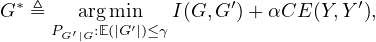
As shown by Theorem 1, the original GIB formulation does
not fully align with the notion of explainability. Consequently,
we adopt the following modified objective function:
where Y ′≜ f(G′) is the predicted label of G′ made by the
model to be explained f, and the cross-entropy CE(Y,Y ′)
between the ground truth label Y and Y ′ is used in place of
H(Y |G′) in the original GIB. The modified GIB avoids the
signaling issues in Theorem 1, by comparing the correct label Y
with the prediction output Y ′ based on the original model f(⋅).
This is in contrast with the original GIB principle which
measures the mutual information I(Y,G′), which provides a
general measure of how well Y can be predicted from G′ (via
Fano’s inequality (El Gamal and Kim 2010)), without relating
this prediction to the original model f(⋅). It should be mentioned
that several recent works have also adopted this modified
GIB formulation (Ying et al. 2019; Luo et al. 2020).
However, the rationale provided in these earlier studies
was that the modified GIB serves as a computationally
efficient approximation for the original GIB, rather than
addressing the limitations of the original GIB shown in Theorem
1.
K-FactExplainer for Graph Neural Networks
In this section, we first theoretically show that existing
parametric explainers based on the GIB objective, such as
PGExplainer (Luo et al. 2020), are subject to two sources of
inaccuracies: locality and lossy aggregation. Then we propose a
straightforward and effective approach to mitigating the
problem. In the subsequent sections, we provide simulation
results that corroborate these theoretical predictions.
Theoretical Analysis
We first define the general class of local explanation methods.
Definition 2 (Geodisc Restricted Graph). Given a graph
G = (,;Z,A), node v ∈, and a radius r ∈ℕ, the
(v,r)-restriction of G is the graph Gv,r = (v,r,v,r;Zv,r,Av,r),
where
-
v,r ≜ {v′|d(v,v′) ≤ r}, where d(⋅,⋅) is the geodisc
distance.
-
v,r ≜{(vi,vj)|e ∈,vi,vj ∈v,r}.
-
Zv,r consists of feature vectors in Z corresponding to
v ∈v,r.
-
Av,r is the adjacency matrix corresponding to v,r.
Definition 3 (Local Explanation Methods). Consider a graph
classification task (,,PG,Y ), a classification function
f : →, a parameter r ∈ℕ, and an explanation function
Ψ : →, where is the set of all possible input graphs, and
is the set of output labels. Let G′ = Ψ(G) = (′,′;Z′,A′).
The explanation function Ψ(⋅) is called an r-local explanation
function if:
-
1.
- The Markov chain 1(v ∈′) ↔ Gv,r ↔ G holds for all
v ∈, where 1(⋅) is the indicator function.
-
2.
- The edge (v,v′) is in ′if and only if v,v′ ∈ ′and
e ∈.
The first condition in Definition 3 requires that the presence
of each vertex v in the explanation G′ only depends on
its neighboring vertices in G which are within its r local
neighborhood. The second condition requires that G′ be a
subgraph of G. It is straightforward to show that various
explanation methods such as PGExplainer are local explanation methods due to the boundedness of their corresponding
computation graphs. This is formalized in the following
proposition.
Proposition 1 (Locality of PGExplainer).
Consider a graph classification task (,,PG,Y ) and an
ℓ layer GNN classifier f(⋅), for some ℓ ∈ ℕ. Then, any
explanation Ψ(⋅) for f(⋅) produced using the PGExplainer
is an ℓ-local explanation function.
Next, we argue that local explanation methods cannot be
optimal in the modified GIB sense for various classification
tasks. Furthermore, we argue that this issue may be mitigated by
the addition of a hyperparameter k as described in subsequent
sections in the context of the K-FactExplainer.
To provide concrete analytical arguments, we focus on a
specific graph classification task, where the class labels
are binary, the input graph has binary-valued edges, and
the output label is a function of a set of indicator motifs.
To elaborate, we assume that the label to be predicted is
Y = max{E1,E2, ,Es}, where Ei,i ∈ [s] are Bernoulli
variables, and if Ei = 1, then gi ⊆ G for some fixed subgraphs
gi,i ∈ [s]. In the explainability literature, each of the subgraphs
gi,i ∈ [s] is called a motif for label Y = 1. Let us define
Ge = ⋃
i∈[s]gi1(Ei = 1). So that Ge is the union of all the
edges in the motifs that are present in G, and it is empty if
Y = 0. Formally, the classification task under consideration is
characterized by the following joint distribution:
,Es}, where Ei,i ∈ [s] are Bernoulli
variables, and if Ei = 1, then gi ⊆ G for some fixed subgraphs
gi,i ∈ [s]. In the explainability literature, each of the subgraphs
gi,i ∈ [s] is called a motif for label Y = 1. Let us define
Ge = ⋃
i∈[s]gi1(Ei = 1). So that Ge is the union of all the
edges in the motifs that are present in G, and it is empty if
Y = 0. Formally, the classification task under consideration is
characterized by the following joint distribution:
where es ∈{0,1}s, ge ≜⋃
i∈[s]gi1(ei = 1), and G0 is the
“irrelevant” edges in G with respect to the label Y .
Remark 4. The graph classification task on the MUTAG
dataset is an instance of the above classification scenario,
where there are two motifs, corresponding to the existence
of NH2 and NO2 chemical groups, respectively (Ying
et al. 2018). Similarly, the BA-4Motif classification task
considered in the Appendix can be posed in the form of
equation 4.
In graph classification tasks characterized by equation 4, if
the label of G is one, then at least one of the motifs is present in
G. Note that the reverse may not be true as the motifs may
randomly appear in the ‘irrelevant’ graph G0 due to its
probabilistic nature. A natural choice for the explanation
function Ψ(⋅) of a classifier f(⋅) for this task is one which
outputs one of the motifs present in G if f(G) = 1. For instance,
in the MUTAG classification task, an explainer should output
NH2 or NO2 subgraphs if the output label is equal to
one. In the following, we argue that, in classification tasks
involving more than one motif local explanation methods
cannot produce the motifs accurately. Hence their output
does not align with the natural explanation outlined above
and is not optimal in the modified GIB sense. To make the
result concrete, we further make the following simplifying
assumptions:
i) The graph G0 is Erdös-Rényi with parameter p ∈ (0, ):
):
ii) There exists r,r′ > 0 such that the geodisc radius and
geodisc diameter of gi are less than or equal to r and r′,
respectively, for all i ∈ [s].
iii) The geodisc distance between gi and gj is greater than r
for all i≠j.
iv) Ei,i ∈ [s] are jointly independent Bernoulli variables with
parameter pi, where PG0(gi) ≤ pi.
Theorem 2 (Suboptimality of Local Explanation Functions).
Let r,r′∈ℕ. For the graph classification task described in
equation 4, the following hold:
a) The optimal Bayes classification rule f*(g) is equal to
1(∃i ∈ [s] : gi ⊆ g).
b) For any r-local explanation function, there exists α′ > 0
such that the explanation is suboptimal for f* in the
modified GIB sense for all α > α′and γ equal to maximum
number of edges of gi,i ∈ [s].
c) There exists an integer k ≤ s, a parameter α′ > 0, a
collection of r′-local explanation functions Ψi(⋅),i ∈ [k],
and an explanation function Ψ*, such that for all inputs g,
we have Ψ(g) ∈ {Ψ1(g),Ψ2(g), ,Ψk(g)} and Ψ* is
optimal in the modified GIB sense for all α > α′ and γ
equal to maximum number of edges of gi,i ∈ [s].
,Ψk(g)} and Ψ* is
optimal in the modified GIB sense for all α > α′ and γ
equal to maximum number of edges of gi,i ∈ [s].
The proof of Theorem 2 is provided in the Appendix.
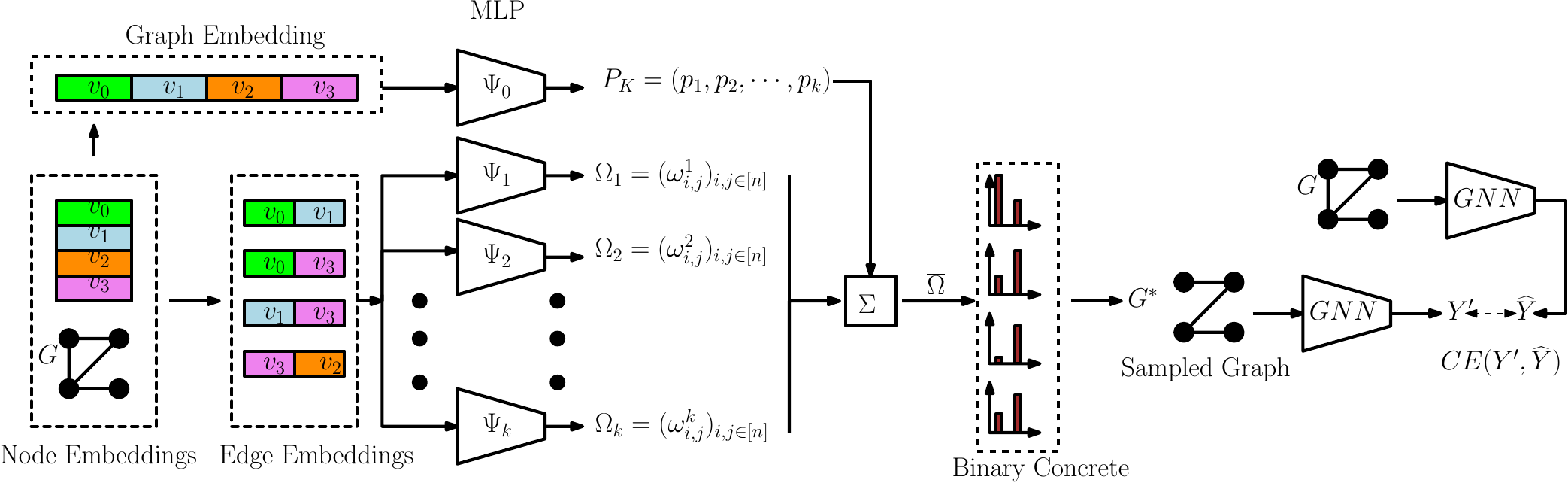
Figure 1: Illustration of K-FactExplainer method. Starting from the left, the node embeddings for graph G are produced
using the original GNN. The edge embeddings and graph embedding are produced by concatenating the node embeddings.
The MLP Ψ0 assigns weight to the outputs of PGExplainer MLPs Ψt,t ∈ [k]. The resulting vector of edge probabilities
Ω ≜ (∑
t=1kptωi,jt)i,j∈[n] is used to produce the sampled explanation graph G*. The explanation is fed to the original GNN
and the output label is compared with the original prediction. The training proceeds by minimizing the cross-entropy term
CE(Y ′, ), where
  is GNN prediction for the original input graph G.
Theorem 2 can be interpreted as follows: for graph classification
tasks with more than one motif, although local explanation
methods are not optimal in general, one can “patch” together
several local explanation methods Ψ1(⋅),Ψ2(⋅), ,Ψk(⋅) into
an explanation method Ψ*(⋅), such that i) for any given input g,
the output of Ψ*(g) is equal to the output of one of the
explanation functions Ψ1(g),Ψ2(g),
,Ψk(⋅) into
an explanation method Ψ*(⋅), such that i) for any given input g,
the output of Ψ*(g) is equal to the output of one of the
explanation functions Ψ1(g),Ψ2(g), ,Ψk(g), and ii) Ψ*(⋅) is
optimal in the modified GIB sense. This insight motivates
the K-FactExplainer method introduced in the following
section.
,Ψk(g), and ii) Ψ*(⋅) is
optimal in the modified GIB sense. This insight motivates
the K-FactExplainer method introduced in the following
section.
Remark 5. Theorem 2 implies that local explanation
methods are not optimal in multi-motif classification tasks.
It should be noted that even in single-motif tasks, post-hoc
methods which rely on GNN generated node embeddings
for explanations would perform suboptimally. The reason
is that the aggregator function which is used to generate
the embeddings is lossy (is not a one-to-one function) and
potentially loses information during the GNN aggregation
step. This can also be observed in the simulation results
provided in the sequel, where we apply our proposed
K-FactExplainer method and show gains compared to
the state of the art in both multi-motif and single-motif
scenarios.
K-FactExplainer and a Bootstrapping Algorithm
Motivated by the insights gained by the analytical results in the
previous section, we propose a new graph explanation method.
An overview of the proposed method is shown in Figure 1. To
describe the method, let f(⋅) be the GNN which we wish to
explain. Let Zi,i ∈ [n] denote the node embedding for
node vi,i ∈ [n] produced by f(⋅). We construct the edge
embeddings Zi,j = (Zi,Zj),i,j ∈ [n] and graph embedding
Z = (Zi,i ∈ [n]) by concatenating the edge embeddings. Let
k ∈ℕ be the upper-bound on the number of necessary local
explainers from Theorem 2. We consider k multi-layer neural
networks (MLPs) denoted by Ψt,t ∈ [k]. Each MLP Ψt
individually operates in a similar fashion as the MLP used in the
PGExplainer method. That is, Ψt operates on each edge
embedding (Zi,Zj) individually, and outputs a Bernoulli
parameter ωi,jt ∈ [0,1]. The parameter ωi,jt ∈ [0,1] can be
viewed as the probability that the edge (vi,vj) is in the sampled
explanation graph. Based on the insights provided by Theorem
2, we wish to patch together the outputs of Ψt,t ∈ [k] to
overcome the locality issue in explaining GNNs in multi-motif
classification tasks. This is achieved by including the additional
MLP Ψ0 which takes the graph embedding Z as input and
outputs the probability distribution PK on the alphabet [k].
At a high level, the MLP Ψ0 provides a global view of
the input graph, whereas each of the Ψt,t ∈ [k] MLPs provide a local perspective of the input graph. The outputs
(ωi,jt)i,j∈[n] of Ψt are linearly combined with weights
associated with PK(t),t ∈ [k] and the resulting vector of
Bernoulli probabilities Ω = (∑
t=1kPK(t)ωi,jt)i,j∈[n] is used
to sample the edges of the input graph G and produce the
explanation graph G*. In the training phase, G* is fed to f(⋅) to
produce the prediction Y ′. Training is performed by minimizing
the cross-entropy term CE(Y ′, ), where
  = f(G) is
the label prediction of the GNN given input G. The next
proposition provides an algorithm to bound the value of k,
which determines the number of MLPs which need to be
trained.
= f(G) is
the label prediction of the GNN given input G. The next
proposition provides an algorithm to bound the value of k,
which determines the number of MLPs which need to be
trained.
|
|
|
|
|
|
|
| | BA-Shapes | BA-Community | Tree-Circles | Tree-Grid | BA-2motifs | MUTAG |
|
|
|
|
|
|
|
| GRAD | 0.882 | 0.750 | 0.905 | 0.667 | 0.717 | 0.783 |
| ATT | 0.815 | 0.739 | 0.824 | 0.612 | 0.674 | 0.765 |
| RGExp. | 0.985±0.013 | 0.919±0.017 | 0.787±0.099 | 0.927±0.032 | 0.657±0.107 | 0.873±0.028 |
| DEGREE | 0.993±0.005 | 0.957±0.010 | 0.902±0.022 | 0.925±0.040 | 0.755±0.135 | 0.773±0.029 |
|
|
|
|
|
|
|
| GNNExp. | 0.742±0.006 | 0.708±0.004 | 0.540±0.017 | 0.714±0.002 | 0.499±0.004 | 0.606±0.003 |
| PGExp. | 0.999±0.000 | 0.825±0.040 | 0.760±0.014 | 0.679±0.008 | 0.566±0.004 | 0.843±0.162 |
|
|
|
|
|
|
|
| K-FactExplainer | 1.000±0.000 | 0.974±0.004 | 0.779±0.004 | 0.770±0.004 | 0.821±0.005 | 0.915±0.010 |
|
|
|
|
|
|
|
| |
Table 1: Explanation faithfulness in terms of AUC-ROC on edges under six datasets. The higher, the better. Our approach
achieves consistent improvements over GIB-based explanation methods.
Proposition 2 (Bounding the Number of MLPs).
Consider the setup in Theorem 2. The parameter k, the
number of r′-local explainers needed to achieve optimal
GIB performance, can be upper-bounded by k*if Ge has a
minimal r′-cover with k*elements.
Particularly, if the classifier to be explained, f(⋅), is a GNN
with ℓ layers, and ℓ is greater than or equal to the largest
geodisc diameter of the motifs gi,i ∈ [s], then k can be
upper-bounded by s.
The proof of Proposition 2 is provided in the Appendix.
Proposition 2 provides a method to find an upper-bound on k;
however, it requires that the motifs be known beforehand, so that
Ge is known and the size of its minimal cover can be computed.
In practice, we do not know the motifs before the start of the
explanation process, since the explanation task would be trivial
otherwise. We provide an approximate solution, where instead of
finding the minimal cover for Ge, we use a bootstrapping
method in which we find the minimal cover for the explanation
graphs produced by another pre-trained explainer, e.g., a
PGExplainer. To elaborate, It takes the GNN model to be
explained f, a set of training input graphs G, and a post-hoc
explainer Ψ as input. In our simulations, we adopt PGExplainer
as the post-hoc explainer Ψ. Other explanation methods such as
GNNExplainer (Ying et al. 2019) can also be used in this step.
For each graph G ∈G, we first apply the explainer Ψ on G to get
the initial explanation graph, whose nodes are listed in Ve
and edge mask matrix is denoted by M. This is used as an
estimate for Ge. To find its minimal cover, we rank the
nodes in Ve based on their degrees and initialize k′ = 0.
For each step, we select a node v from Ve and extract its
k*-hop neighborhood graph, Gv(l). Then, we remove all
nodes in Gv(l) from Ve. After that, we add a count to k′
and select the next node in Ve until |Ve| = 0. We iterate
all graphs in G and report the maximum value of k′ as  ,
the estimate of k. A detailed algorithm can be found in
Appendix.
,
the estimate of k. A detailed algorithm can be found in
Appendix.
Related Work
Graph neural networks (GNNs) have gained increasing attention
in recent years due to the need for analyzing graph data
structures (Kipf and Welling 2017; Veličković et al. 2018; Xu
et al. 2019; Feng et al. 2020; Satorras, Hoogeboom, and
Welling 2021; Bouritsas et al. 2022). In general, GNNs model
messages from node representations and then propagate
messages with message-passing mechanisms to update
representations. GNNs have been successfully applied in various
graph mining tasks, such as node classification (Kipf and
Welling 2017), link prediction (Zhang and Chen 2018), and
graph classification (Xu et al. 2019). Despite their popularity,
akin to other deep learning methodologies, GNNs operate as
black box models, which means their functioning can be hard to
comprehend, even when the message passing techniques and
parameters used are known. Furthermore, GNNs stand apart
from conventional deep neural networks that assume instances
are identically and independently distributed. GNNs instead
integrate node features with graph topology, which complicates
the interpretability issue.
Recent studies have aimed to interpret GNN models and offer
explanations for their predictions (Ying et al. 2019; Luo
et al. 2020; Yuan et al. 2020, 2022, 2021; Lin, Lan, and
Li 2021; Wang and Shen 2023; Miao et al. 2023; Fang
et al. 2023; Ma et al. 2022; Zhang, Luo, and Wei 2023). These
methods generally fall into two categories based on granularity:
i) instance-level explanation (Ying et al. 2019; Zhang
et al. 2022), which explains predictions for each instance by
identifying significant substructures; and ii) model-level
explanation (Yuan et al. 2020; Wang and Shen 2023; Azzolin
et al. 2023), designed to understand global decision rules
incorporated by the target GNN. Among these methods, Post-hoc
explanation ones (Ying et al. 2019; Luo et al. 2020; Yuan
et al. 2021), which employ another model or approach to
explain a target GNN. Post-hoc explanations have the advantage
of being model-agnostic, meaning they can be applied to a
variety of GNNs. Therefore, our work focuses on post-hoc
instance-level explanations (Ying et al. 2019), that is,
identifying crucial instance-wise substructures for each input to
explain the prediction using a trained GNN model. A detailed
survey can be found in (Yuan et al. 2022).
|
|
|
|
|
|
|
| | BA-Shapes | BA-Community | Tree-Circles | Tree-Grid | BA-2motifs | MUTAG |
|
|
|
|
|
|
|
| PGExp. | 0.999±0.000 | 0.825±0.040 | 0.760±0.014 | 0.679±0.008 | 0.566±0.004 | 0.843±0.162 |
| k = 1 | 1.000±0.000 | 0.850±0.047 | 0.758±0.023 | 0.711±0.011 | 0.580±0.041 | 0.769±0.119 |
| k = 2 | 1.000±0.000 | 0.880±0.023 | 0.779±0.018 | 0.707±0.570 | 0.581±0.039 | 0.801±0.105 |
| k = 3 | 1.000±0.000 | 0.902±0.022 | 0.772±0.012 | 0.710±0.005 | 0.586±0.034 | 0.895±0.034 |
| k = 5 | 1.000±0.000 | 0.899±0.011 | 0.768±0.013 | 0.709±0.006 | 0.573±0.044 | 0.892±0.030 |
| k = 10 | 1.000±0.000 | 0.926±0.012 | 0.774±0.006 | 0.706±0.004 | 0.578±0.039 | 0.915±0.021 |
| k = 20 | 1.000±0.000 | 0.938±0.013 | 0.778±0.006 | 0.704±0.002 | 0.586±0.032 | 0.911±0.014 |
| k = 60 | 1.000±0.000 | 0.952±0.011 | 0.778±0.004 | 0.770±0.004 | 0.588±0.030 | 0.915±0.010 |
|
|
|
|
|
|
|
| |
Table 2: Explanation performances w.r.t. k. We use underlines to denote k selected by the proposed method.
Experimental Study
In this section, we empirically verify the effectiveness and
efficiency of the proposed K-FactExplainer by explaining both
node and graph classifications. We also conduct extensive
studies to verify our theoretical claims. Due to the space
limitation, detailed experimental setups, full experimental
results, and extensive experiments are presented in Appendix.
|
|
|
|
|
|
|
|
|
| | k = 1 | k = 2 | k = 3 | k = 5 | k = 10 | k = 20 | k = 60 | |
|
|
|
|
|
|
|
|
|
| BA-Community(20) | 0.850 | 0.880 | 0.902 | 0.899 | 0.926 | 0.938 | 0.952 | |
| BA-Community(80) | 0.893 | 0.899 | 0.895 | 0.894 | 0.895 | 0.895 | 0.897 | |
|
|
|
|
|
|
|
|
|
| Tree-Circles(20) | 0.758 | 0.779 | 0.772 | 0.768 | 0.774 | 0.778 | 0.778 | |
| Tree-Circles(80) | 0.871 | 0.871 | 0.871 | 0.870 | 0.871 | 0.871 | 0.870 | |
|
|
|
|
|
|
|
|
|
| |
Table 3: Effects of lossy aggregation on GNNs with different hidden layer sizes
Experimental Setup.
We compare our method with representative GIB-based
explanation methods, GNNExplainer (Ying et al. 2019)
and PGExplainer (Luo et al. 2020), classic explanation
methods, GRAD (Ying et al. 2019) and ATT (Veličković
et al. 2018), and SOTA methods, RG-Explainer (Shan
et al. 2021) and DEGREE (Feng et al. 2022). We follow the
routinely adopted framework to set up our experiments (Ying
et al. 2019; Luo et al. 2020). Six benchmark datasets with
ground truth explanations are used for evaluation, with
BA-Shapes, BA-Community, Tree-Circles, and Tree-Grid (Ying
et al. 2019) for the node classification task, and BA-2motifs (Luo
et al. 2020) and MUTAG (Debnath et al. 1991) for the graph
classification task. For each dataset, we train a graph neural
network model to perform the node or graph classification task.
Each model is a three-layer GNN with a hidden size of
20, followed by an MLP that maps these embeddings to
the number of classes. After training the model, we apply
the K-FactExplainer and the baseline methods to generate
explanations for both node and graph instances. For each
experiment, we conduct 10 times with random parameter
initialization and report the average results as well as the
standard deviation. Detailed experimental setups are put in the
appendix.
Quantitative Evaluation
Comparison to Baselines.
We adopted the well-established experimental framework (Ying
et al. 2019; Luo et al. 2020; Shan et al. 2021), where the
explanation problem is framed as a binary classification of edges.
Within this setup, edges situated inside motifs are regarded as
positive edges, while all others are treated as negative. The
importance weights offered by the explanation methods
are treated as prediction scores. An effective explanation
method, therefore, would assign higher weights to edges
located within the ground truth motifs as opposed to those
outside. To quantitatively evaluate the performance of these
methods, we employed AUC as our metric. The average AUC
scores and the associated standard deviations are reported in
Table 1. We observe that with a manually selected value for k,
K-FactExplainer consistently outperforms GNNExplainer and
PGExplainer and competes with high-performing models like
RGExplainer and DEGREE. The comparison demonstrates that
our K-FactExplainer considers locality, providing more accurate,
comprehensive explanations and mitigating common locality
pitfalls seen in other models.
Model Analysis
Effectiveness of Bootstrapping Algorithm.
To directly show the effects of k in K-FactExplainer . We change
the value of k from 1 to 60 and show the resulting performance
in Table 2. We observe that, in general, a higher value of k leads
to improved performance. The reason is that large k in
K-FactExplainer mitigates the locality and lossy aggregation
losses in parametric explainers as discussed previously. We use
an underline to indicate the upper-bound for the value of
k suggested by the bootstrap algorithm in Section 0.0.
It should be noted that this upper-bound is particularly
relevant to multi-motif scenarios considered in Theorem 2.
Restricting to values of k that are less than or equal to the
suggested upper-bound achieves the best performance in the
multi-motif MUTAG task, which is aligned with our theoretical
analysis.
Effects of Lossy Aggregation.
To evaluate the effects of lossy aggregation, we consider the
BA-Community and Tree-Cycles in this part. As shown
in Table 2, K-FactExplainer significantly outperforms
PGExplainer. The reason is that the K-FactExplainer partially
mitigates the aggregation loss in GNN explanation methods by
combining the outputs of multiple MLPs, hence combining
multiple ‘weak’ explainers into a stronger one. In addition,
we observe that the performances of K-FactExplainer are
positively related to k. Next, we increase the dimensionality of
hidden representation in the GNN model from 20 to 80. This
reduces the loss in aggregation as at each layer several low
dimensional vectors are mapped to high dimensional vectors.
The explanation performances are shown in Table 3. For these
two datasets, the performance improves as k is increased when
the dimension is 20, due to the mitigation of the aggregation
loss, however, as expected, no improvement is observed when
increasing k in explaining the GNN with dimension 80, since
there is no significant aggregation loss to mitigate in that
case.
Conclusion
In this work, we theoretically investigate the trivial solution
problem in the popular objective function for explaining
GNNs, which is largely overlooked by the existing post-hoc
instance-level explanation approaches. We point out that
the trivial solution is caused by the signal problem and
propose a new GIB objective with a theoretical guarantee. On
top of that, we further investigate the locality and lossy
aggregation issues in existing parametric explainers and
show that most of them can be unified within the local
explanation Methods, which are weak at handling real-world
graphs, where the mapping between labels and motifs is
one-to-many. We propose a new factorization-based explanation
model to address these issues. Comprehensive experiments
are conducted to verify the effectiveness of the proposed
method.
Acknowledgments
This project was partially supported by NSF grants IIS-2331908
and CCF-2241057. The views and conclusions contained in this
paper are those of the authors and should not be interpreted as
representing any funding agencies.
References
Abid, A.; Balin, M. F.; and Zou, J. 2019. Concrete
Autoencoders for Differentiable Feature Selection and
Reconstruction. arXiv:1901.09346.
Azzolin, S.; Longa, A.; Barbiero, P.; Liò, P.; and
Passerini, A. 2023. Global explainability of gnns via
logic combination of learned concepts. In Proceedings of
the International Conference on Learning Representations
(ICLR).
Bouritsas, G.; Frasca, F.; Zafeiriou, S.; and Bronstein,
M. M. 2022. Improving graph neural network expressivity
via subgraph isomorphism counting. IEEE Transactions on
Pattern Analysis and Machine Intelligence, 45(1): 657–668.
Chereda, H.; Bleckmann, A.; Kramer, F.; Leha, A.;
and Beißbarth, T. 2019. Utilizing Molecular Network
Information via Graph Convolutional Neural Networks to
Predict Metastatic Event in Breast Cancer. Studies in health
technology and informatics, 267: 181–186.
Debnath, A. K.; Lopez de Compadre, R. L.; Debnath,
G.; Shusterman, A. J.; and Hansch, C. 1991.
Structure-activity relationship of mutagenic aromatic and
heteroaromatic nitro compounds. correlation with molecular
orbital energies and hydrophobicity. Journal of medicinal
chemistry, 34(2): 786–797.
El Gamal, A.; and Kim, Y.-H. 2010. Lecture notes on
network information theory.
Fan, W.; Ma, Y.; Li, Q.; He, Y.; Zhao, Y.; Tang, J.;
and Yin, D. 2019. Graph Neural Networks for Social
Recommendation. The World Wide Web Conference.
Fang, J.; Wang, X.; Zhang, A.; Liu, Z.; He, X.; and
Chua, T.-S. 2023. Cooperative Explanations of Graph
Neural Networks. In Proceedings of the Sixteenth ACM International Conference on Web Search and Data Mining,
616–624.
Feng, Q.; Liu, N.; Yang, F.; Tang, R.; Du, M.; and Hu,
X. 2022. DEGREE: Decomposition Based Explanation for
Graph Neural Networks. In International Conference on
Learning Representations.
Feng, W.; Zhang, J.; Dong, Y.; Han, Y.; Luan, H.; Xu,
Q.; Yang, Q.; Kharlamov, E.; and Tang, J. 2020. Graph
random neural networks for semi-supervised learning on
graphs. Advances in neural information processing systems,
33: 22092–22103.
Kipf, T. N.; and Welling, M. 2017. Semi-Supervised
Classification with Graph Convolutional Networks. In
International Conference on Learning Representations.
Li, J.; Cheng, K.; Wang, S.; Morstatter, F.; Trevino,
R. P.; Tang, J.; and Liu, H. 2017. Feature selection: A data
perspective. ACM computing surveys (CSUR), 50(6): 1–45.
Lin, W.; Lan, H.; and Li, B. 2021. Generative causal
explanations for graph neural networks. In International
Conference on Machine Learning, 6666–6679. PMLR.
Liu, Z.; Yang, L.; Fan, Z.; Peng, H.; and Yu, P. S.
2022. Federated social recommendation with graph neural
network. ACM Transactions on Intelligent Systems and
Technology (TIST), 13(4): 1–24.
Lu, Z.; Lv, W.; Xie, Z.; Du, B.; Xiong, G.; Sun, L.; and
Wang, H. 2022. Graph Sequence Neural Network with an
Attention Mechanism for Traffic Speed Prediction. ACM
Transactions on Intelligent Systems and Technology (TIST),
13(2): 1–24.
Luo, D.; Cheng, W.; Xu, D.; Yu, W.; Zong, B.; Chen,
H.; and Zhang, X. 2020. Parameterized explainer for graph
neural network. Advances in neural information processing
systems, 33: 19620–19631.
Ma, J.; Guo, R.; Mishra, S.; Zhang, A.; and Li, J.
2022. CLEAR: Generative Counterfactual Explanations on
Graphs. In Proceedings of Advances in neural information
processing systems.
Mansimov, E.; Mahmood, O.; Kang, S.; and Cho,
K. 2019. Molecular Geometry Prediction using a Deep
Generative Graph Neural Network. Scientific Reports, 9.
Miao, S.; Liu, M.; and Li, P. 2022. Interpretable
and generalizable graph learning via stochastic attention
mechanism. In International Conference on Machine
Learning, 15524–15543. PMLR.
Miao, S.; Luo, Y.; Liu, M.; and Li, P. 2023. Interpretable
Geometric Deep Learning via Learnable Randomness
Injection. In Proceedings of the International Conference
on Learning Representations (ICLR).
Satorras, V. G.; Hoogeboom, E.; and Welling, M. 2021.
E (n) equivariant graph neural networks. In International
conference on machine learning, 9323–9332. PMLR.
Shan, C.; Shen, Y.; Zhang, Y.; Li, X.; and Li, D.
2021. Reinforcement Learning Enhanced Explainer for
Graph Neural Networks. Advances in Neural Information
Processing Systems, 34.
Tishby, N.; and Zaslavsky, N. 2015. Deep learning
and the information bottleneck principle. In 2015 ieee
information theory workshop (itw), 1–5. IEEE.
Veličković, P.; Cucurull, G.; Casanova, A.; Romero, A.;
Liò, P.; and Bengio, Y. 2018. Graph Attention Networks. In
International Conference on Learning Representations.
Wang, X.; and Shen, H.-W. 2023. GNNInterpreter:
A Probabilistic Generative Model-Level Explanation for
Graph Neural Networks. In Proceedings of the International
Conference on Learning Representations (ICLR).
Wang, X.; Wu, Y.; Zhang, A.; He, X.; and Chua, T.-S.
2021. Towards multi-grained explainability for graph neural
networks. Advances in Neural Information Processing
Systems, 34: 18446–18458.
Wu, T.; Ren, H.; Li, P.; and Leskovec, J. 2020. Graph
information bottleneck. Advances in Neural Information
Processing Systems, 33: 20437–20448.
Xu, K.; Hu, W.; Leskovec, J.; and Jegelka, S. 2019. How Powerful are Graph Neural Networks? In International
Conference on Learning Representations.
Ying, R.; He, R.; Chen, K.; Eksombatchai, P.; Hamilton,
W. L.; and Leskovec, J. 2018. Graph convolutional neural
networks for web-scale recommender systems. In KDD,
974–983.
Ying, Z.; Bourgeois, D.; You, J.; Zitnik, M.; and
Leskovec, J. 2019. Gnnexplainer: Generating explanations
for graph neural networks. In NeurIPS, 9240–9251.
Yu, J.; Xu, T.; Rong, Y.; Bian, Y.; Huang, J.; and
He, R. 2021. Graph Information Bottleneck for Subgraph
Recognition. In International Conference on Learning
Representations.
Yuan, H.; Tang, J.; Hu, X.; and Ji, S. 2020. Xgnn:
Towards model-level explanations of graph neural networks.
In Proceedings of the 26th ACM SIGKDD International
Conference on Knowledge Discovery & Data Mining,
430–438.
Yuan, H.; Yu, H.; Gui, S.; and Ji, S. 2022. Explainability
in graph neural networks: A taxonomic survey. IEEE
Transactions on Pattern Analysis and Machine Intelligence.
Yuan, H.; Yu, H.; Wang, J.; Li, K.; and Ji, S. 2021.
On explainability of graph neural networks via subgraph
explorations. In International Conference on Machine
Learning, 12241–12252. PMLR.
Zhang, J.; Luo, D.; and Wei, H. 2023. MixupExplainer:
Generalizing Explanations for Graph Neural Networks with
Data Augmentation. In Proceedings of the 29th ACM
SIGKDD Conference on Knowledge Discovery and Data
Mining, 3286–3296.
Zhang, M.; and Chen, Y. 2018. Link prediction based
on graph neural networks. Advances in neural information
processing systems, 31.
Zhang, S.; Liu, Y.; Shah, N.; and Sun, Y. 2022. Gstarx:
Explaining graph neural networks with structure-aware
cooperative games. Advances in Neural Information
Processing Systems, 35: 19810–19823.
Appendix
Proofs
Proof of Lemma 1
Note that from the data processing inequality and B ↔ C ↔ A′,
we have:
Also, from PA|C = PA′|C, we have:
Lastly, from A ↔ B ↔ C, we have:
Combining these three results, we get:
| I(A′,B) ≤ I(A′,C) = I(A,C) ≤ I(A,B). | | |
__
Proof of Theorem 1
Let us define γα ≜ minG′I(G,G′) + αH(Y |G′), and let Gα*
be an explanation achieving γα. Define G′α as a random graph
generated conditioned on h(G) such that PG′α|h(G) = PGα*|h(G)
and the Markov chain G,Gα* ↔ h(G) ↔ G′α holds.
It can be observed that by construction the conditions in
Lemma 1 are satisfied for A ≜ Gα*,A′≜ G′α,B ≜ G and
C ≜ h(G). Hence, we have I(G′α,G) ≤ I(Gα*,G). As a
result:
| γα = I(G,Gα*) + αH(Y |G
α*) |  I(G,G′α) + αH(Y |Gα*) I(G,G′α) + αH(Y |Gα*) | |
|
|  I(G,G′α) + αH(Y |G′α) I(G,G′α) + αH(Y |G′α) | | |
where in (a) follows from I(G′α,G) ≤ I(Gα*,G)
and (b) follows from the fact that the task is statistically
degraded, the Markov chain Gα*G′α ↔ h(G) ↔ Y and
PGα*|h(G) = PG′α|h(G). Consequently, G′α is also an
optimal explanation in the GIB sense, i.e. achieves γα. The
proof is completed by defining the explanation function as
Ψα(G) = G′α. __
Proof of Theorem 2
Part a): Note that the optimal Bayes classifier rule is given by
f*(g) = arg maxy∈{0,1}P(y|G = g). If ∄i ∈ [s] : gi ⊆ g, then
P(Y = 1|G = g) = 0 and hence f*(g) = 0 as desired.
So, it suffices to show that if ∃i ∈ [s] : gi ⊆ g, then
P(Y = 1|G = g) > P(Y = 0|G = g). Let  = {i ∈ [s]|gi ⊆ g}.
Note that
= {i ∈ [s]|gi ⊆ g}.
Note that
| P(Y = 1|G = g) > P(Y = 0|G = g) ⇐⇒ | |
|
| P(G = g,Y = 1) > P(G = g,Y = 0). | | |
Also,
| P(G = g,Y = 1) |  ∏
i∈ ∏
i∈ P(gi ⊆ Ge)P(g -∪i∈gi ⊆ G0 ⊆ g) P(gi ⊆ Ge)P(g -∪i∈gi ⊆ G0 ⊆ g) | |
|
|  (∏
i∈pi)P(g -∪i∈gi ⊆ G0 ⊆ g) (∏
i∈pi)P(g -∪i∈gi ⊆ G0 ⊆ g) |
(5) |
where (a) follows from the facts that i) if all indicator motifs
are equal to one then Y = 1, ii) the indicator motifs are
independent of each other, and iii) Ge and G0 are independent of
each other, and (b) follows from the fact that the indicator motifs
are Bernoulli variables with parameters pi,i ∈ [s]. On the other
hand:
| P(G = g,Y = 0) P(G0 = g) P(G0 = g) | |
|
|  ∏
i∈P(gi ⊆ G0)P(g -∪i∈gi = G0 -∪i∈gi), ∏
i∈P(gi ⊆ G0)P(g -∪i∈gi = G0 -∪i∈gi), | | |
where (a) follows from the fact that if Y = 1 all indicator
motifs are equal to zero, and in (b) we have used the fact that the
graph G0 is Erdös-Rényi, and the motif subgraphs do not
overlap. So,
| P(G = g,Y = 0) ≤ (∏
i∈pi)P(g -∪i∈gi ⊆ G0 ⊆ g), | |
(6) |
where we have used the fact that from condition iv) in the
problem formulation, we have P(gi ⊆ G0) ≤ pi,i ∈ [s].
Combining equation 5 and equation 6 completes the proof of
a).
Part b): We provide an outline of the proof. It can be observed
that as α →∞, the optimal explanation algorithm in the
modified GIB sense is the one that minimized the cross-entropy
term CE(Y,Y ′). We argue that the optimal explanation
algorithm outputs one of the motifs present in g if Y = 1.
The reasons is that in this case, f*(g) = f*(Ψ(g)) for all
input graphs g, and the cross-entropy term is minimized
by the assumption that f* is the optimal Bayes classifier
rule.
Next, we argue that an r-local explanation method cannot
produce the optimal explanation. The reason is that due to
condition ii) and iii) in the problem formulation and definition of
r-local explanation methods, the probability that an edge in a
given motif is included in the explanation only depends on the
presence of the corresponding motif in graph g and not the
presence of the other motifs. To see this, let pj,j′ be the
probability that the edge (vj,vj′) in motif gi ⊆ g is included in
the explanation Ψ(g). Then, by linearity of expectation, we
have:
So, we must have:
Consequently, the r-local explanation method cannot output
one of the motifs present in g with probability one since the edge
probabilities pj,j′ cannot be equal to one as their summation
should be less than γ. This completes the proof of part
b).
Part c): We construct an optimal explainer as follows. Let k = s
and define Ψi(g) ≜ gi1(gi ∈ g). Furthermore, define the
explainer Ψ*(g) ≜ arg mingi,i∈[s]{i|gi ⊆ g}. Then, since for
Y = 1, the output of Ψ* is a motif that is present in the input
graph, as explained in the proof of Part b), Ψ(g) is an optimal
explanation function in the modified GIB sense as α →∞ as
it yields the minimum cross-entropy term. Furthermore,
Ψ(g) ∈{Ψ1(g),Ψ2(g), ,Ψk(g)} by construction. This
completes the proof. __
,Ψk(g)} by construction. This
completes the proof. __
Proof of Proposition 2
Following the arguments in the proof of Theorem 2,
it suffices to show that there exist Ψt,t ∈ [k*] and
Ψ(⋅) ∈{Ψ1(⋅),Ψ2(⋅), ,Ψk*(⋅)}, such that Ψ(g) is equal to a
motif that is present in g whenever Y = 1. To construct such an
explainer, let P = {
,Ψk*(⋅)}, such that Ψ(g) is equal to a
motif that is present in g whenever Y = 1. To construct such an
explainer, let P = { t,t ∈ [k*]} be the minimal k*-cover of Ge,
and let gi* be the motif in the input graph with the smallest index
among all motifs present in the input graph. We take Ψt,t ∈ [k*]
to be such that it assigns sampling probability one to the edges in
t belonging to the motif gi in the input graph with the smallest
index among all motifs whose edges overlap with t and
sampling probability zero to every other edge, i.e. it outputs the
motif with the smallest index in its computation graph with
probability one. Let Ψ0 be such that it assigns probability one to
an Ψt,t ∈ [k*] for which t overlaps with gi* and zero
to all other Ψt. Then, it is straightforward to see that the
resulting sampled graph from K-FactExplainer G* would
be equal to the motif with the smallest index among the
motifs present in the input graph gi*. This completes the
proof. __
t,t ∈ [k*]} be the minimal k*-cover of Ge,
and let gi* be the motif in the input graph with the smallest index
among all motifs present in the input graph. We take Ψt,t ∈ [k*]
to be such that it assigns sampling probability one to the edges in
t belonging to the motif gi in the input graph with the smallest
index among all motifs whose edges overlap with t and
sampling probability zero to every other edge, i.e. it outputs the
motif with the smallest index in its computation graph with
probability one. Let Ψ0 be such that it assigns probability one to
an Ψt,t ∈ [k*] for which t overlaps with gi* and zero
to all other Ψt. Then, it is straightforward to see that the
resulting sampled graph from K-FactExplainer G* would
be equal to the motif with the smallest index among the
motifs present in the input graph gi*. This completes the
proof. __
Algorithm
The detailed algorithm for Bootstrapping is shown in Alg. 1.
Algorithm 1: Bootstrapping Algorithm to Bound the
Number of MLPs
Require: the GNN model to be explained,
f, a set of graphs
G, an explainer
Ψ.
1:  ← 0
← 0.
2: for each graph
G = (,,X,A) ∈G do
3: M ← Ψ(f,G) # get a mask of edges by applying g
to explain f on G.
4: m ←  # get all node in the
explanation graphs.
# get all node in the
explanation graphs.
5: Ve ←{vi|mi > 0} # get all node in the explanation
graphs.
6: Rank the nodes in Ve according to their
degrees/betweenness.
7: k′← 0
8: while Ve is not empty do
9: get a node v from Ve with smallest degree;
10: Gv(l) ← l-hop neighborhood graph with v.
11: remove nodes of Gv(l) from Ve
12: k′← k′ + 1
13: end while
14:  ← max(k′,
 ).
15: end for
16: return
).
15: end for
16: return 
Detailed Experimental Setups
Experimental Setup
In the experimental study, we first describe the synthetic and
real-world datasets used for experiments, baseline methods, and
experimental setup. After qualitative and quantitative analysis,
we demonstrate that the K-FactExplainer is effective for
explaining both node and graph instances, and it outperforms
state-of-the-art explanation methods in various scenarios. We
attribute the gains of K-FactExplainer to the mitigation
of two types of performance losses, which were studied
analytically in prior sections, namely, lossy aggregation and
locality.
As mentioned in Remark 5, the first type of loss, aggregation
loss, is due to the fact that the aggregator function at each layer
of the GNN is not one-to-one, and hence loses information. This
is particularly true if the mid-layers of the GNN have similar
(low) dimensions. The second type of loss, the locality loss,
manifests in multi-motif scenarios as shown in Theorem 2. In
order to study each of these types of losses in isolation, we first
focus on single-motif tasks and study lossy aggregation,
then, we focus on multi-motif tasks and study the locality
loss.
To prove that the explainer’s performance gains in single-motif
tasks are indeed due to the mitigation of aggregation loss, it
suffices to show that if the lossy aggregator is replaced by a
(almost) lossless aggregator, the performance gains vanish. One
can construct a GNN with almost lossless aggregation by
choosing the dimensionality of the layers of the GNN to be
sequentially increasing. Hence, to demonstrate our claim, we
consider several single-motif classification tasks and show that
increasing the hyperparameter k leads to performance gains if
the GNN has similar low-dimensional mid-layers, whereas if the
layers increase in dimension sequentially, no performance
gain is observed when increasing k, thus confirming the
hypothesis that the K-FactExplainer gains in single-motif
scenarios are indeed due to lossy aggregation. To demonstrate
the fact that the K-FactExplainer mitigates the locality
loss suffered by conventional local explainers, we consider
several multi-motif classification tasks, and show that the
explainer’s accuracy increases as k is increased in accordance
with the analytical results of Theorem 2 and Algorithm
1.
Datasets.
Six benchmark datasets are used for evaluation, with BA-Shapes,
BA-Community, Tree-Circles, and Tree-Grid (Ying et al. 2019)
for the node classification task, and BA-2motifs (Luo et al. 2020)
and MUTAG (Debnath et al. 1991) for the graph classification
task. BA-Shapesis a dataset generated using the Barabási-Albert
(BA) graph randomly attached with “house”-structured network motifs. BA-Community, also generated using the BA model,
focuses on community structures within the graph, with
nodes connected based on a preferential attachment model.
Tree-Circlesis a dataset where cycle structures are embedded
within trees, created by introducing cycles by connecting nodes
in the trees. Lastly, Tree-Gridis a dataset that combines tree and
grid structures by embedding grid structures within trees.
MUTAG is a real-world dataset that comprises chemical
compound graphs, where each graph represents a chemical
compound, and the task is to predict whether the compound is
mutagenic or not. These synthetic and real datasets allow us to
evaluate the performance of the K-FactExplainer and baseline
methods in controlled settings, providing insights into their
effectiveness and interpretability for node classification
tasks.
Baselines.
To assess the effectiveness of the proposed framework,
we compare our method with representative GIB-based
explanation methods, GNNExplainer (Ying et al. 2019) and
PGExplainer (Luo et al. 2020). We also include other types of
explanation methods, RG-Explainer (Shan et al. 2021) and
DEGREE (Feng et al. 2022), GRAD (Ying et al. 2019), and
ATT (Veličković et al. 2018) for comparison. Specifically,
GRAD computes gradients of GNN’s objective function w.r.t.
each edge for its importance score. (2) ATT averages the edge
attention weights across all layers to compute the edge weights.
(3) GNNExplainer (Ying et al. 2019) is a post-hoc method,
which provides explanations for every single instance by
learning an edge mask for the edges in the graph. The weight of
the edge could be treated as important. (4) PGExplainer (Luo
et al. 2020) extends GNNExplainer by adopting a deep neural
network to parameterize the generation process of explanations,
which enables PGExplainer to explain the graphs in a global
view. It also generates the substructure graph explanation
with the edge importance mask. (5) RGExplainer (Shan
et al. 2021) is an RL-enhanced explainer for GNN, which
constructs the explanation subgraph by starting from a seed and
sequentially adding nodes with an RL agent. (6) DEGREE
(Feng et al. 2022) is a decomposition-based approach that
monitors the feedforward propagation process in order to trace
the contributions of specific elements from the input graph to the
final prediction.
For each dataset, we train a graph neural network model to
perform the node or graph classification task. Each model is a
three-layer GNN with a hidden size of 20, followed by an MLP
that maps these embeddings to the number of classes. After
training the model, we apply the K-FactExplainer and the
baseline methods to generate explanations for both node and
graph instances. For each experiment, we conduct 10 times with
random parameter initialization and report the average results as
well as the standard deviation.
Extra Experiments
Model Analysis
Effects of Locality in Multi-motif Tasks. So far, we have
illustrated the gains due to the mitigation of the locality loss by
considering the multi-motif MUTAG classification task (Table
1). To further empirically demonstrate these gains, in this
section, we introduce a new graph classification dataset,
BA-4motifs which includes 1000 stochastically generated
graphs. The generation process follows the procedure described
in equation 4. That is, for each graph, we first generate a base
graph g0 according to the BA model. Then, the graph is assigned
a binary label randomly and uniformly (by generating Es, the
indicators of different motifs). Each label is associated with two
motifs. The motif graph (ge in equation 4) is generated based on
Es, and finally the graph g is produced by taking the union of g0
and ge.
As shown in Theorem 2, assuming that the classifier to be
explained has optimal performance, the optimal explainer (in the
modified GIB sense) outputs one of the motifs that are present in
the graph. Consequently, we define the motif coverage rate (CR)
as a measure of the performance of the explainer as follows.
Recall that the explainer assigns a probability of being
part of the explanation to each of the graph edges, e.g.,
the probability vector Ω in Figure 1. Let r denote the r
top-ranked edges in terms of probability of being part of the
explanation, where r is the maximum motif size. For each
motif gi ∈ g with edge set i, we define its coverage rate as
CRi ≜ , i.e., the fraction of the motif’s edges that are
top-ranked. The CR is defined as maxiCRi, the maximum of
coverage rate among all motifs. Table 4 shows that with more
complex datasets, our method will significantly improve
the faithfulness of the explanation in terms of coverage
rate.
, i.e., the fraction of the motif’s edges that are
top-ranked. The CR is defined as maxiCRi, the maximum of
coverage rate among all motifs. Table 4 shows that with more
complex datasets, our method will significantly improve
the faithfulness of the explanation in terms of coverage
rate.
Table 4: Average Coverage Rate for BA-4motifs.
|
|
|
|
|
|
| | GNNExp. | PGExp. | k=1 | k=2 | k=3 |
|
|
|
|
|
|
| Coverage Rate (CR) | 0.114 | 0.433 | 0.442 | 0.615 | 0.712 |
| AUC | 0.737 | 0.755 | 0.761 | 0.772 | 0.789 |
|
|
|
|
|
|
| |
Efficiency Analysis
The proposed method comprises networks capable of generating
inductive explanations for new instances across a population.
Following (Luo et al. 2020), we measure the inference time,
which is the time needed to explain a new instance with a trained
model. Table 5 presents the running time for K-FactExplainer
with various K values. The results indicate that the inference
time of K-FactExplainer is comparably similar to that of the
PGExplainer, which is one of the most sufficient explanation
techniques.
|
|
|
|
|
|
|
| | BA-Shapes | BA-Community | Tree-Circles | Tree-Grid | BA-2motifs | MUTAG |
|
|
|
|
|
|
|
| PGExp. | 4.27 | 6.48 | 0.50 | 0.55 | 0.44 | 2.48 |
| K=1 | 4.18 | 6.16 | 0.46 | 0.53 | 0.44 | 3.01 |
| K=2 | 4.26 | 6.26 | 0.49 | 0.57 | 0.47 | 2.50 |
| K=3 | 4.47 | 6.88 | 0.55 | 0.62 | 0.55 | 2.86 |
| K=5 | 4.27 | 6.29 | 0.53 | 0.58 | 0.52 | 2.56 |
| K=10 | 4.39 | 6.42 | 0.58 | 0.69 | 0.53 | 2.78 |
| K=20 | 4.69 | 6.81 | 0.66 | 0.85 | 0.65 | 3.17 |
| K=60 | 5.75 | 8.39 | 1.38 | 1.20 | 1.14 | 5.79 |
|
|
|
|
|
|
|
| |
Table 5: K-Explainer Inference Time (ms)
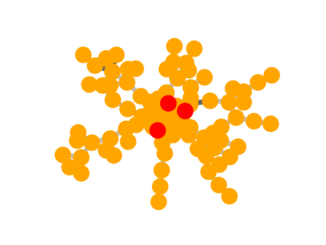
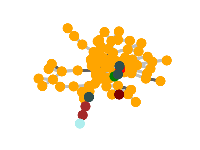
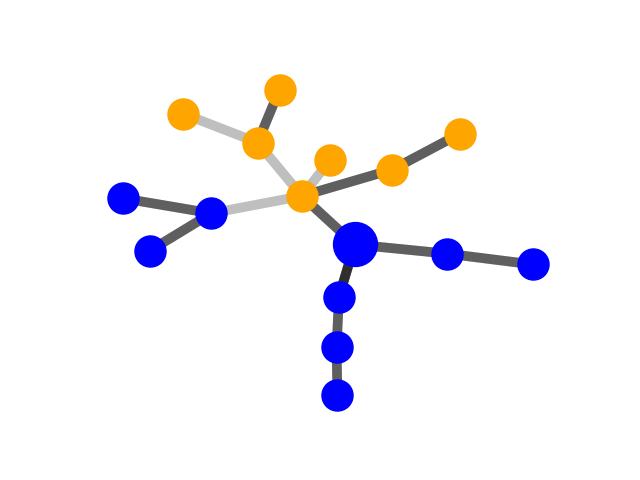
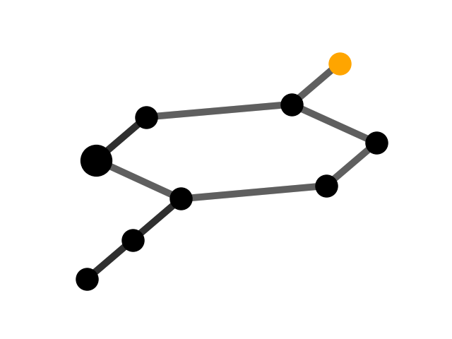
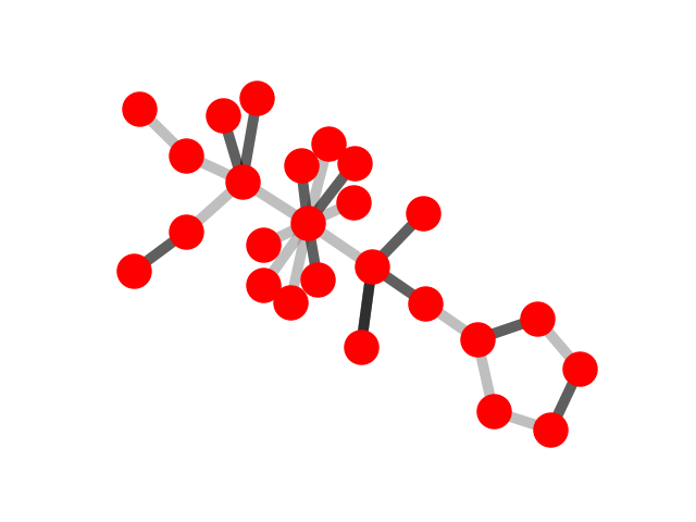
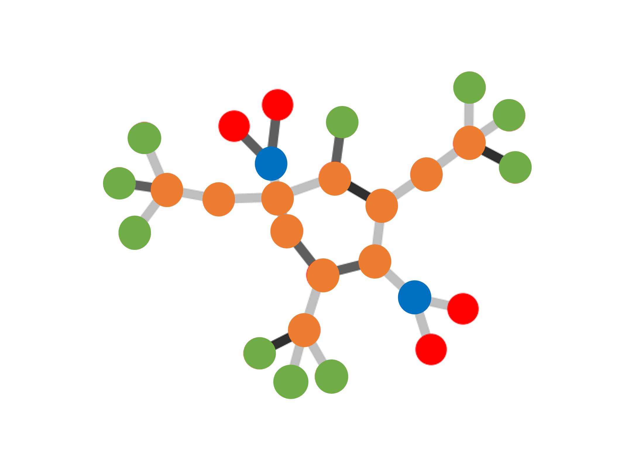
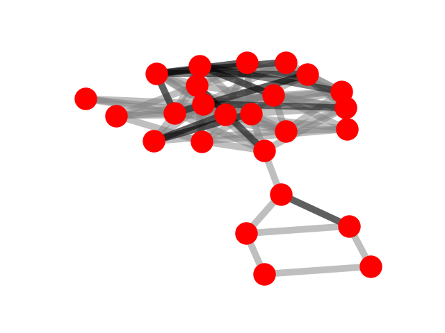
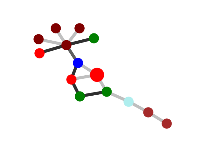
Qualitative evaluation
We selected an instance to visually demonstrate the explanations
given by GNNExplainer, PGExplainer, and K-FactExplainer in
Table 6.
Table 6: Qualitative Analysis

![P (g,y)
∑G,Y
= PEs(es)PG0(g0)1(y = mia∈x[s] ei,g = g0 ∪ge),
es,g0](cameraReady7x.png)