Local Community Detection in Multiple Networks
Dongsheng Luo1*, Yuchen Bian2*, Yaowei Yan1, Xiao Liu1, Jun Huan3, Xiang Zhang1
1Pennsylvania State University, 2NEC Labs America, 3StylingAI Inc.
{dul262,yxy230,xxl213,xzz89}@psu.edu,yuchenbian@baidu.com,lukehuan@shenshangtech.com
Abstract
Local community detection aims to find a set of densely-connected nodes containing given query nodes. Most existing local community detection methods are designed for a single network. However, a single network can be noisy and incomplete. Multiple networks are more informative in real-world applications. There are multiple types of nodes and multiple types of node proximities. Complementary information from different networks helps to improve detection accuracy. In this paper, we propose a novel RWM (Random W alk in Multiple networks) model to find relevant local communities in all networks for a given query node set from one network. RWM sends a random walker in each network to obtain the local proximity w.r.t. the query nodes (i.e., node visiting probabilities). Walkers with similar visiting probabilities reinforce each other. They restrict the probability propagation around the query nodes to identify relevant subgraphs in each network and disregard irrelevant parts. We provide rigorous theoretical foundations for RWM and develop two speeding-up strategies with performance guarantees. Comprehensive experiments are conducted on synthetic and real-world datasets to evaluate the effectiveness and efficiency of RWM.
1 Introduction
As a fundamental task in large network analysis, local community detection has attracted extensive attention recently. Unlike the time-consuming global community detection, the goal of local community detection is to detect a set of nodes with dense connections (i.e., the target local community) that contains a given query node or a query node set [1, 2, 4, 6, 7, 15, 17, 29, 33].
Most existing local community detection methods are designed for a single network. However, a single network may contain noisy edges and miss some connections which results in unsatisfactory performance. On the other hand, in real-life applications, more informative multiple network structures are often constructed from different sources or domains [18, 20, 22, 25, 28].
(a)
Co-worker |
(b)
Lunch-together |
(c)
Facebook-friends |
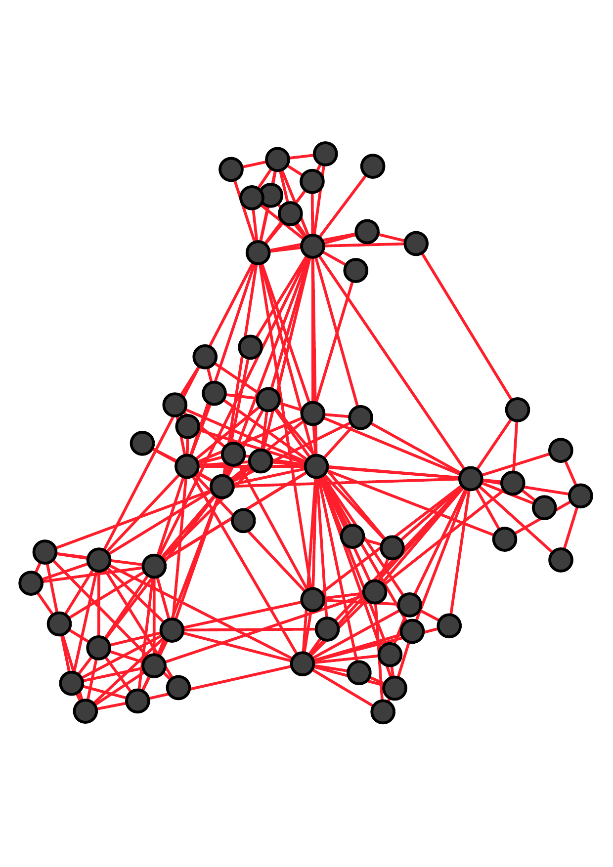
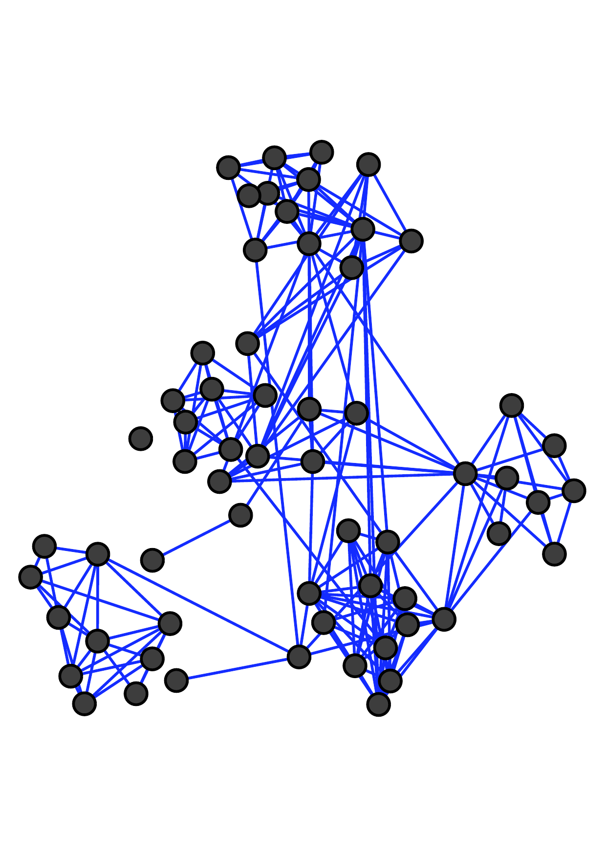
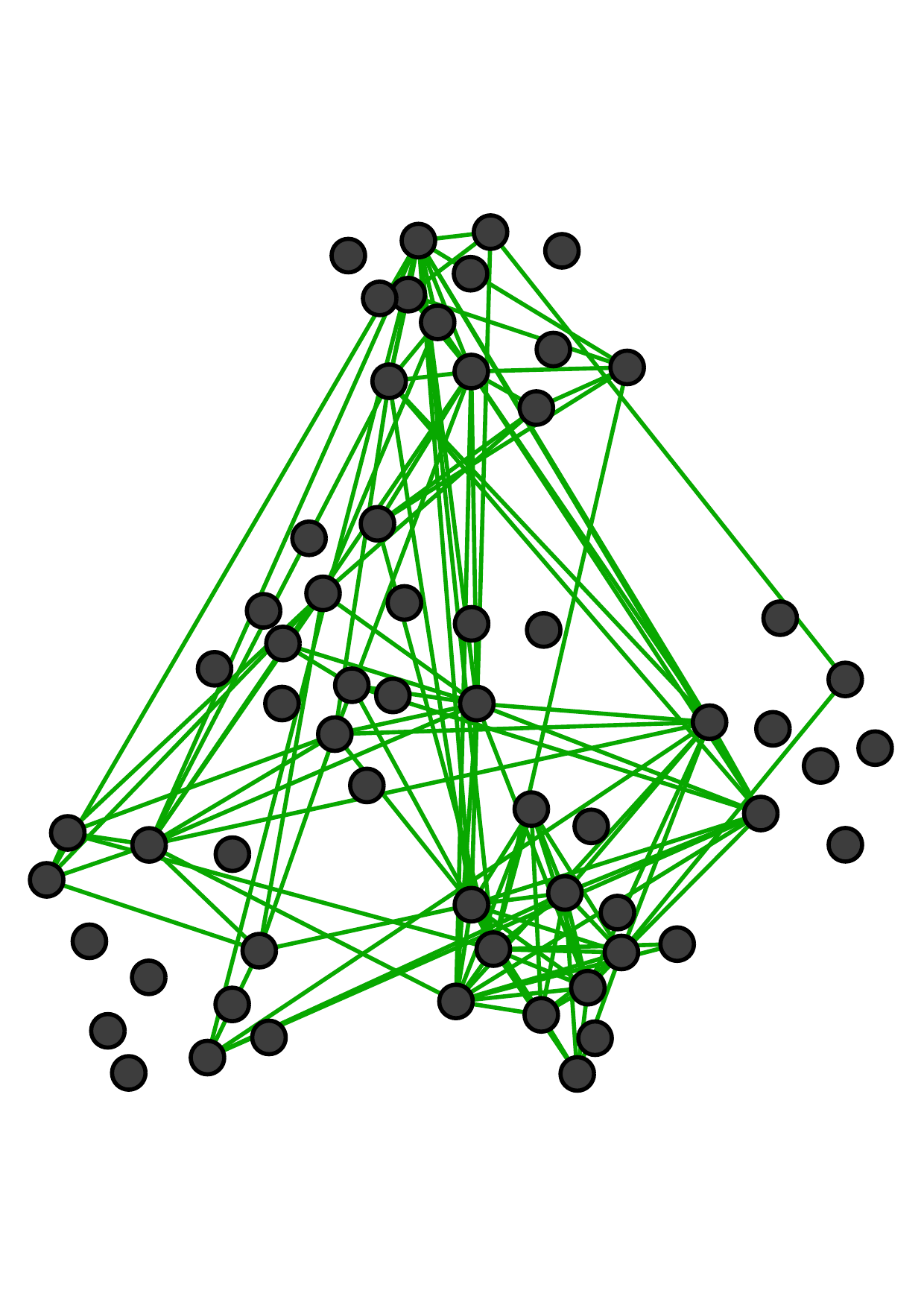
There are two main kinds of multiple networks. Fig. 1 shows an example of multiple networks with the same node set and different types of edges (which is called multiplex networks [14, 21] or multi-layer network). Each node represents an employee of a university [13]. These three networks reflect different relationships between employees: co-workers, lunch-together, and Facebook-friends. Notice that more similar connections exist between two off-line networks (i.e., co-worker and lunch-together) than that between the off-line and online relationships (i.e., Facebook-friends).
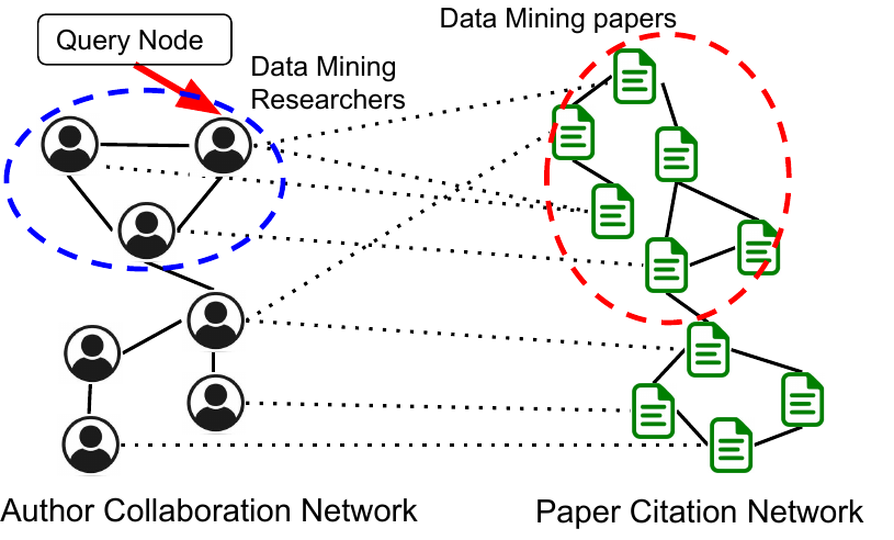
Fig. 2 is another example from the DBLP dataset with multiple domains of nodes and edges (which is called multi-domain networks [22]). The left part is the author-collaboration network and the right part is the paper-citation network. A cross-edge connecting an author and a paper indicates that the author writes the paper. We see that authors and papers in the same research field may have dense cross-links. Suppose that we are interested in one author, we want to find both the relevant author community as well as the paper community, which includes papers in the research field of the query author. Then cross-edges can provide complementary information from the query (author) domain to other domains (paper) and vise versa. Detecting relevant local communities in two domains can enhance each other.
Note that multiplex networks are a special case of multi-domain networks with the same set of nodes and the cross-network relations are one-to-one mappings. Few works discuss local community detection in comprehensive but complicated multiple networks. Especially, no existing work can find query-relevant local communities in all domains in the more general multi-domain networks.
In this paper, we focus on local community detection in multiple networks. Given a query node in one network, our task is to detect a query-relevant local community in each network.
A straightforward method is to independently find the local community in each network. However, this baseline only works for the special multiplex networks and cannot be generalized to multi-domain networks. In addition, this simple approach does not consider the complementary information in multiple networks (e.g., similar local structures among the three relations in Fig. 1).
In this paper, we propose a random walk based method, RWM (Random W alk in Multiple networks), to find query-relevant local communities in multiple networks simultaneously. The key idea is to integrate complementary influences from multiple networks. We send out a random walker in each network to explore the network topology based on corresponding transition probabilities. For networks containing the query node, the probability vectors of walkers are initiated with the query node. For other networks, probability vectors are initialized by transiting visiting probability via cross-connections among networks. Then probability vectors of the walkers are updated step by step. The vectors represent walkers’ visiting histories. Intuitively, if two walkers share similar or relevant visiting histories (measured by cosine similarity and transited with cross-connections), it indicates that the visited local typologies in corresponding networks are relevant. And these two walkers should reinforce each other with highly weighted influences. On the other hand, if visited local typologies of two walkers are less relevant, smaller weights should be assigned. We update each walker’s visiting probability vector by aggregating other walkers’ influences at each step. In this way, the transition probabilities of each network are modified dynamically. Comparing with traditional random walk models where the transition matrix is time-independent [2, 15, 17, 30, 31], RWM can restrict most visiting probability in the most query-relevant subgraph in each network and ignore irrelevant or noisy parts.
Theoretically, we provide rigorous analyses of the convergence properties of the proposed model. Two speeding-up strategies are developed as well. We conduct extensive experiments on real and synthetic datasets to demonstrate the advantages of our RWM model on effectiveness and efficiency for local community detection in multiple networks.
Our contributions are summarized as follows.
-
We propose a novel random walk model, RWM, to detect local communities in multiple networks for a given query node set. Especially, based on our knowledge, this is the first work which can detect all query-relevant local communities in all networks for the general multi-domain networks.
-
Fast estimation strategies and sound theoretical foundations are provided to guarantee effectiveness and efficiency of RWM.
-
Results of comprehensive experiments on synthetic and real multiple networks verify the advances of RWM.
2 Related Work
Local community detection is one of the cutting-edge problems in graph mining. In a single network, local search based method [23, 28], flow-based method [29], and subgraph cohesiveness-optimization based methods, such as 𝑘-clique [24, 36], 𝑘-truss [9, 11], 𝑘-core [3] are developed to detect local communities. A recent survey about local community detection and community search can be found in [10].
Except for that, random walk based methods have also been routinely applied to detect local communities in a single network [2, 5, 8, 15, 32, 34, 35]. A walker explores the network following the topological transitions. The node visiting probability is usually utilized to determine the detection results. For example, PRN [2] runs the lazy random walk to update the visiting probability and sweeps the ranking list to find the local community with the minimum conductance. The heat kernel method applies the heat kernel coefficients as the decay factor to find small and dense communities [15]. In [35], the authors propose a motif-based random walk model and obtain node sets with the minimal motif conductance. MWC [5] sends multiple walkers to explore the network to alleviate the query-bias issue. Note that all aforementioned methods are designed for a single network.
Some methods have been proposed for global community detection in multiple networks. An overview can be found in [13]. However, they focus on detecting all communities, which are time-consuming and are independent of a given query node. Very limited work aim to find query-oriented local communities in multiple networks. For the special case, i.e., multiplex networks, a greedy algorithm is developed to find a community shared by all networks [12]. Similarly, a modified random walk model is proposed in [8] for multiplex networks. For the general multi-domain networks, the method in [34] can only detect one local community in the query network domain. More importantly, these methods assume that all networks share similar or consistent structures. Different from these methods, our method RWM does not make such an assumption. RWM can automatically identify relevant local structures and ignore irrelevant ones in all networks.
3 Random Walk in Multiple Networks
In this section, we first introduce notations. Then the reinforced updating mechanism among random walkers in RWM is proposed. A query-restart strategy is applied in the end to detect the query-relevant local communities in multiple networks.
3.1 Notations. Suppose that there are 𝐾 undirected networks, the 𝑖th (1 ≤𝑖≤𝐾) network is represented by 𝐺𝑖 = (𝑉𝑖 ,𝐸𝑖 ) with node set 𝑉𝑖 and edge set 𝐸𝑖 . We denote its transition matrix as a column-normalized matrix P𝑖 ∈R|𝑉𝑖 |×|𝑉𝑖 |. The (𝑣,𝑢)th entry P𝑖 (𝑣,𝑢) represents the transition probability from node 𝑢 to node 𝑣 in 𝑉𝑖 . Then the 𝑢th column P𝑖 (:,𝑢) is the transition distribution from node 𝑢 to all nodes in 𝑉𝑖 . Next, we denote 𝐸𝑖-𝑗 the cross-connections between nodes in two networks 𝑉𝑖 and 𝑉𝑗 . The corresponding cross-transition matrix is S𝑖→𝑗 ∈R|𝑉𝑗 |×|𝑉𝑖 |. Then the 𝑢th column S𝑖→𝑗 (:,𝑢) is the transition distribution from node 𝑢∈𝑉𝑖 to all nodes in 𝑉𝑗 . Note that S𝑖→𝑗 ≠ S𝑗→𝑖 . And for the multiplex networks with the same node set (e.g., Fig. 1), S𝑖→𝑗 is just an identity matrix I for arbitrary 𝑖,𝑗. Suppose we send a random walker in 𝐺𝑖 , we let x𝑖 (𝑡) be the node visiting probability vector in 𝐺𝑖 at time 𝑡. Then the updated vector x𝑖 (𝑡+1)= P𝑖 x𝑖 (𝑡) means the probability transiting among nodes in 𝐺𝑖 . And S𝑖→𝑗 x𝑖 (𝑡) is the probability vector propagated into 𝐺𝑗 from 𝐺𝑖 .
Given a query node2 𝑢𝑞 in the query network 𝐺𝑞 , the target of local community detection in multiple networks is to detect relevant local communities in all networks 𝐺𝑖 (1 ≤𝑖≤𝐾). Important notations are summarized in Table 1.
| Notation | Definition |
| 𝐾 | The number of networks |
| 𝐺𝑖 = (𝑉𝑖 ,𝐸𝑖 ) | The 𝑖th network with nodes set 𝑉 𝑖 and edge set 𝐸𝑖 |
| P𝑖 | Column-normalized transition matrix of 𝐺𝑖 . |
| 𝐸𝑖-𝑗 | The cross-edge set between network 𝐺𝑖 and 𝐺𝑗 |
| S𝑖→𝑗 | Column-norm. cross-trans. mat. from 𝑉𝑖 to 𝑉𝑗 |
| 𝑢𝑞 | A given query node 𝑢𝑞 from 𝑉𝑞 |
| e𝑞 | One-hot vector with only one value-1 entry for 𝑢𝑞 |
| x𝑖 (𝑡) | Node visit. prob. vec. of the 𝑖th walker in 𝐺𝑖 at 𝑡 |
| W(𝑡) | Relevance weight matrix at time 𝑡 |
| P𝑖 (𝑡) | Modified trans. mat. for the 𝑖th walker in 𝐺𝑖 at 𝑡 |
| α,λ,θ | restart factor, decay factor, covering factor. |
3.2 Reinforced Updating Mechanism. In RWM, we send out one random walker for each network. Initially, for the query node 𝑢𝑞 ∈𝐺𝑞 , the corresponding walker’s x𝑞 (0)= e𝑞 where e𝑞 is a one-hot vector with only one value-1 entry corresponding to 𝑢𝑞 . For other networks 𝐺𝑖 (𝑖≠ 𝑞), we initialize x𝑖 (0) by x𝑖 (0)= S𝑞→𝑖 x𝑞 (0). That is3 :
| (1) |

To update 𝑖th walker’s vector x𝑖 (𝑡), the walker not only follows the transition probabilities in the corresponding network 𝐺𝑖 , but also obtains influences from other networks. Intuitively, networks sharing relevant visited local structures should influence each other with higher weights. And the ones with less relevant visited local structures have fewer effects. We measure the relevance of visited local structures of two walkers in 𝐺𝑖 and 𝐺𝑗 with the cosine similarity of their vectors x𝑖 (𝑡) and x𝑗 (𝑡). Since different networks consist of different node sets, we define the relevance as cos(x𝑖 (𝑡),S𝑗→𝑖 x𝑗 (𝑡)). Notice that when 𝑡 increases, walkers will explore nodes further away from the query node. Thus, we add a decay factor λ(0 <λ<1) in the relevance to emphasize the similarity between local structures of two different networks within a shorter visiting range. In addition, as shown in the theoretical analysis in Appendix4 , λ can guarantee and control the convergence of the RWM model. Formally, we let W(𝑡)∈R𝐾×𝐾 be the local relevance matrix among networks at time 𝑡 and we initialize it with identity matrix I. We update each entry W(𝑡)(𝑖,𝑗) as follow:
| (2) |

For the 𝑖th walker, influences from other networks are reflected in the dynamic modification of the original transition matrix P𝑖 based on the relevance weights. Specifically, the modified transition matrix of 𝐺𝑖 is:
| (3) |

where S𝑗→𝑖 P𝑗 S𝑖→𝑗 represents the propagation flow pattern 𝐺𝑖 →𝐺𝑗 →𝐺𝑖
(counting from the right side) and  (𝑡)(𝑖,𝑗)=
  is the
row-normalized local relevance weights from 𝐺𝑗 to 𝐺𝑖 . To guarantee
the stochastic property of transition matrix, we also column-normalize
P𝑖 (𝑡) after each updating.
is the
row-normalized local relevance weights from 𝐺𝑗 to 𝐺𝑖 . To guarantee
the stochastic property of transition matrix, we also column-normalize
P𝑖 (𝑡) after each updating.
At time 𝑡+1, the visiting probability vector of the walker in 𝐺𝑖 is updated:
| (4) |

Different from the classic random walk model, transition matrices in RWM dynamically evolve with local relevance influences among walkers from multiple networks. As a result, the time-dependent property enhances RWM with the power of aggregating relevant and useful local structures among networks for the local community detection.
Next, we theoretically analyze the convergence properties. First, in Theorem 1, we present the weak convergence property [5] of the modified transition matrix P𝑖 (𝑡). The convergence of the visiting probability vector will be provided in Theorem 3.
Theorem 1. When applying RWM in multiple networks, for any
small tolerance 0 <ϵ<1, for all 𝑖, when 𝑡>⌈log λ  ⌉,
∥P𝑖 (𝑡+1)-P𝑖 (𝑡) ∥∞ <ϵ, where 𝑉𝑖 is the node set of network 𝐺𝑖
and ∥·∥∞is the ∞-norm of a matrix.
⌉,
∥P𝑖 (𝑡+1)-P𝑖 (𝑡) ∥∞ <ϵ, where 𝑉𝑖 is the node set of network 𝐺𝑖
and ∥·∥∞is the ∞-norm of a matrix.
For the multiple networks with the same node set (i.e., multiplex networks), we have a faster convergence rate.
Theorem 2. When applying RWM in multiple networks with
the same node set, for any small tolerance 0 <ϵ<1, for all 𝑖,
∥P𝑖 (𝑡+1)-P𝑖 (𝑡)∥∞<ϵ, when 𝑡>⌈log λ  ⌉.
⌉.
Please refer to the Appendix for the proof details of these theorems. Next, we describe how to detect relevant local communities in multiple networks given a query node from one network.
4 Local Community Detection With Restart Strategy
RWM is a general random walk model for multiple networks and can be further customized into different variations. In this section, we integrate the idea of random walk with restart (RWR) [26] into RWM and use it for local community detection. Note that the original RWR is only for a single network instead of multiple networks.
In RWR, at each time point, the random walker explores the network based on topological transitions with α(0 <α<1) probability and jumps back to the query node with probability 1 -α. The restart strategy enables RWR to obtain proximities of all nodes to the query node.
Similarly, we apply the restart strategy for RWM in updating visiting probability vectors. For the 𝑖th walker, we have:
| (5) |

where P𝑖 (𝑡) is obtained by Eq. (3). Since the restart component does not provide any information for the visited local structure, we dismiss this part when calculating local relevance weights. Therefore, we modify the cos(·,·) in Eq. (2) and have:
| (6) |

Theorem 3. Adding the restart strategy in RWM does not affect the convergence properties in Theorems 1 and 2. The visiting vector x𝑖 (𝑡)(1 ≤𝑖≤𝐾)will also converge.
We skip the proof here. The main idea is that λ first guarantees the weak convergence of P𝑖 (𝑡) (λ has the same effect as in Theorem 1). After obtaining a converged P𝑖 (𝑡), Perron-Frobenius theorem [19] can guarantee the convergence of x𝑖 (𝑡) with a similar convergence proof of the traditional RWR model.
To find the local community in network 𝐺𝑖 , we follow the common process in the literature [2, 5, 15, 34]. We first sort nodes according to the converged score vector x𝑖 (𝑇), where 𝑇 is the number of iterations. Suppose there are 𝐿 non-zero elements in x𝑖 (𝑇), for each 𝑙(1 ≤𝑙≤𝐿), we compute the conductance of the subgraph induced by the top 𝑙 ranked nodes. The node set with the smallest conductance will be considered as the detected local community.
Time complexity of RWM. As a basic method, we can iteratively update vectors until convergence or stop the updating at a given number of iterations 𝑇 . Algorithm 1 shows the overall process.
In each iteration, for the 𝑖th walkers (line 4-5), we update x𝑖 (𝑡+1) based on Eq. (3) and (5) (line 4). Note that we do not compute the modified transition matrix P𝑖 (𝑡) and output. If we substitute Eq. (3) in Eq. (5), we have a probability propagation S𝑗→𝑖 P𝑗 S𝑖→𝑗 x𝑖 (𝑡) which reflects the information flow 𝐺𝑖 →𝐺𝑗 →𝐺𝑖 . In practice, a network is stored as an adjacent list. So we only need to update the visiting probabilities of direct neighbors of visited nodes and compute the propagation from right to left. Then calculating S𝑗→𝑖 P𝑗 S𝑖→𝑗 x𝑖 (𝑡) costs 𝑂(|𝑉𝑖 |+|𝐸𝑖-𝑗 |+|𝐸𝑗 |). And the restart addition in Eq. (5) costs 𝑂(|𝑉𝑖 |). As a result, line 4 costs 𝑂(|𝑉𝑖 |+|𝐸𝑖 |+∑ 𝑗≠𝑖 (|𝐸𝑖-𝑗 |+|𝐸𝑗 |)) where 𝑂(|𝐸𝑖 |) is from the propagation in 𝐺𝑖 itself.
In line 5, based on Eq. (6), it takes 𝑂(|𝐸𝑖-𝑗 |+|𝑉𝑗 |) to get S𝑗→𝑖 x𝑗 (𝑡) and 𝑂(|𝑉𝑖 |) to compute cosine similarities. Then updating W(𝑖,𝑗) (line 5) costs 𝑂(|𝐸𝑖-𝑗 |+|𝑉𝑖 |+|𝑉𝑗 |). In the end, normalization (line 6) costs 𝑂(𝐾2) which can be ignored.
In summary, with 𝑇 iterations, power iteration method for RWM costs 𝑂((∑ 𝑖 |𝑉𝑖 |+∑ 𝑖 |𝐸𝑖 |+∑ 𝑖≠𝑗 |𝐸𝑖-𝑗 |)𝐾𝑇). For the multiplex networks with the same node set 𝑉 , the complexity shrinks to 𝑂((∑ 𝑖 |𝐸𝑖 |+𝐾|𝑉|)𝐾𝑇) because of the one-to-one mappings in 𝐸𝑖-𝑗 .
Note that power iteration methods may propagate probabilities to the entire network which is not a true “local” method. Next, we present two speeding-up strategies to restrict the probability propagation into only a small subgraph around the query node.
 (0) = I;
2for 𝑡←0 to 𝑇 do
3
4
5for 𝑖←1 to 𝐾 do
6
7
8calculate x𝑖 (𝑡+1)according to Eq. (3) and (5);
9calculate W(𝑡+1)according to Eq. (6);
10
(0) = I;
2for 𝑡←0 to 𝑇 do
3
4
5for 𝑖←1 to 𝐾 do
6
7
8calculate x𝑖 (𝑡+1)according to Eq. (3) and (5);
9calculate W(𝑡+1)according to Eq. (6);
10 (𝑡+1)←row-normalize W(𝑡+1);_____________________________________________________
5 Speeding Up
In this section, we introduce two approximation methods which not only dramatically improve the computational efficiency but also guarantee performances.
5.1 Early Stopping. With the decay factor λ, the modified transition matrix of each network converges before the visiting score vector does. Thus, we can approximate the transition matrix with early stopping by splitting the computation into two phases. In the first phase, we update both transition matrices and score vectors, while in the second phase, we keep the transition matrices static and only update score vectors. Now we give the error bound between the early-stopping updated transition matrix and the power-iteration updated one. In 𝐺𝑖 , we denote P𝑖 (∞) the converged modified transition matrix.
In 𝐺𝑖 (1 ≤𝑖≤𝐾), when properly selecting the split time 𝑇𝑒 , the following theorem demonstrates that we can securely approximate the power-iteration updated matrix P𝑖 (∞) with P𝑖 (𝑇𝑒 ).
Theorem 4. For a given small tolerance ϵ, when 𝑡>𝑇𝑒 =
⌈log λ  ⌉, ∥ P𝑖 (∞) -P𝑖 (𝑡) ∥ ∞ <ϵ. For the multiplex
networks with the same node set, we can choose 𝑇𝑒 = ⌈log λ
⌉, ∥ P𝑖 (∞) -P𝑖 (𝑡) ∥ ∞ <ϵ. For the multiplex
networks with the same node set, we can choose 𝑇𝑒 = ⌈log λ  ⌉
to get the same estimation bound ϵ.
⌉
to get the same estimation bound ϵ.
Please refer to Appendix for the proof.
The time complexity of the first phase is 𝑂((∑ 𝑖 |𝑉𝑖 |+∑ 𝑖 |𝐸𝑖 |+∑ 𝑖≠𝑗 |𝐸𝑖-𝑗 |)𝐾𝑇𝑒 ).
 𝑖 (𝑡+1)
1initialize an empty queue 𝑞𝑢𝑒;
2initialize a zero vector x𝑖0(𝑡)with the same size with x𝑖 (𝑡);
3𝑞𝑢𝑒.push(𝑄) where 𝑄is the node set with positive values in x𝑖 (0); mark
nodes in 𝑄as visited;
4𝑐𝑜𝑣𝑒𝑟←0;
5while 𝑞𝑢𝑒is not empty and 𝑐𝑜𝑣𝑒𝑟<θ do
6
7
8𝑢←𝑞𝑢𝑒.pop();
9mark 𝑢as visited;
10for each neighbor node 𝑣of 𝑢 do
11
12
13if 𝑣is not marked as visited then
14
15
16𝑞𝑢𝑒.push(𝑣);
17x𝑖0(𝑡)[𝑢]←x𝑖 (𝑡)[𝑢];
18𝑐𝑜𝑣𝑒𝑟←𝑐𝑜𝑣𝑒𝑟+x𝑖 (𝑡)[𝑢];
19Update
𝑖 (𝑡+1)
1initialize an empty queue 𝑞𝑢𝑒;
2initialize a zero vector x𝑖0(𝑡)with the same size with x𝑖 (𝑡);
3𝑞𝑢𝑒.push(𝑄) where 𝑄is the node set with positive values in x𝑖 (0); mark
nodes in 𝑄as visited;
4𝑐𝑜𝑣𝑒𝑟←0;
5while 𝑞𝑢𝑒is not empty and 𝑐𝑜𝑣𝑒𝑟<θ do
6
7
8𝑢←𝑞𝑢𝑒.pop();
9mark 𝑢as visited;
10for each neighbor node 𝑣of 𝑢 do
11
12
13if 𝑣is not marked as visited then
14
15
16𝑞𝑢𝑒.push(𝑣);
17x𝑖0(𝑡)[𝑢]←x𝑖 (𝑡)[𝑢];
18𝑐𝑜𝑣𝑒𝑟←𝑐𝑜𝑣𝑒𝑟+x𝑖 (𝑡)[𝑢];
19Update  𝑖 (𝑡+1)based on Eq. (7);________________________________________________________________
5.2 Partial Updating. In this section, we propose a heuristic strategy to further speed up the vector updating in Algorithm 1 (line 4) by only updating a subset of nodes that covers most probabilities. Specifically, given a covering factor θ∈(0,1], for walker 𝑖, in the 𝑡th iteration, we separate x𝑖 (𝑡) into two non-negative vectors, x𝑖0(𝑡) and Δx𝑖 (𝑡), so that x𝑖 (𝑡)= x𝑖0(𝑡)+Δx𝑖 (𝑡), and ∥x𝑖0(𝑡)∥1 ≥θ. Then, we approximate x𝑖 (𝑡+1) with
 𝑖 (𝑡+1)= αP𝑖 (𝑡)x𝑖0(𝑡)+(1 -α∥x𝑖0(𝑡)∥1)x𝑖 (0) 𝑖 (𝑡+1)= αP𝑖 (𝑡)x𝑖0(𝑡)+(1 -α∥x𝑖0(𝑡)∥1)x𝑖 (0) | (7) |
Thus, we replace the updating operation of x𝑖 (𝑡+1) in Algorithm 1
(line 4) with  𝑖 (𝑡+1). The details are shown in Algorithm 2. Intuitively,
nodes close to the query node have higher scores than nodes far away.
Thus, we utilize the breadth-first search (BFS) to expand x𝑖0(𝑡) from
the query node set until ∥x𝑖0(𝑡)∥1 ≥θ (lines 3-12). Then, in line 13,
we approximate the score vector in the next iteration according to Eq.
(7).
𝑖 (𝑡+1). The details are shown in Algorithm 2. Intuitively,
nodes close to the query node have higher scores than nodes far away.
Thus, we utilize the breadth-first search (BFS) to expand x𝑖0(𝑡) from
the query node set until ∥x𝑖0(𝑡)∥1 ≥θ (lines 3-12). Then, in line 13,
we approximate the score vector in the next iteration according to Eq.
(7).
Let 𝑉𝑖0(𝑡) be the set of nodes with positive values in x𝑖0(𝑡), and |𝐸𝑖0(𝑡)| be the summation of out-degrees of nodes in 𝑉𝑖0(𝑡). Then |𝐸𝑖0(𝑡)|≪|𝐸𝑖 | which dramatically reduces the number of nodes to update in each iteration.
6 Experiments
We perform comprehensive experimental studies to evaluate the effectiveness and efficiency of the proposed methods. Our algorithms are implemented with C++. The code and data used in this work are available.5 All experiments are conducted on a PC with Intel Core I7-6700 CPU and 32 GB memory, running 64 bit Windows 10.
| Dataset | #Net. | #Nodes |
|
|
|
||||||
| RM | 10 | 910 | 14,289 | – | 40.5 | ||||||
| BrainNet | 468 | 123,552 | 619,080 | – | 14.8 | ||||||
| 6-NG | 5 | 4,500 | 9,000 | 20,984 | 150 | ||||||
| 9-NG | 5 | 6,750 | 13,500 | 31,480 | 150 | ||||||
| Citeseer | 3 | 15,533 | 56,548 | 11,828 | 384.2 | ||||||
| DBLP | 2 | 3,359,321 | 8,723,940 | 5,851,893 | 38.6 | ||||||
Datasets. Six real-world datasets are used to evaluate the effectiveness of the selected methods. Statistics are summarized in Table 2. The first two are multiplex networks with the same node set.
• RM [13] has 10 networks, each with 91 nodes. Nodes represent phones and one edge exists if two phones detect each other under a mobile network. Each network describes connections between phones in a month. Phones are divided into two communities according to their owners’ affiliations.
• BrainNet [27] has 468 brain networks, one for each participant. In the brain network, nodes represent human brain regions and an edge depicts the functional association between two regions. Different participants may have different functional connections. Each network has 264 nodes, among which 177 nodes are studied to belong to 12 high-level functional systems, including auditory, memory retrieval, visual , etc.. Each functional system is considered as a community.
The other four are general multiple networks with different types of nodes and edges and many-to-many cross-edges between nodes in different networks.
• 6-NG & 9-NG [22] are two multi-domain network datasets constructed from the 20-Newsgroup dataset6 . 6-NG contains 5 networks of sizes {600, 750, 900, 1050, 1200} and 9-NG consists of 5 networks of sizes {900, 1125, 1350, 1575, 1800}. Nodes represent news documents and edges describe their semantic similarities. The cross-network relationships are measured by cosine similarity between two documents from two networks. Nodes in the five networks in 6-NG and 9-NG are selected from 6 and 9 news groups, respectively. Each news group is considered as a community.
• Citeseer [18] is from an academic search engine, Citeseer. It contains a researcher collaboration network, a paper citation network, and a paper similarity network. The collaboration network has 3,284 nodes (researchers) and 13,781 edges (collaborations). The paper citation network has 2,035 nodes (papers) and 3,356 edges (paper citations). The paper similarity network has 10,214 nodes (papers) and 39,411 edges (content similarity). There are three types of cross-edges: 2,634 collaboration-citation relations, 7,173 collaboration-similarity connections, and 2,021 citation-similarity edges. 10 communities of authors and papers are labeled based on research areas.
• DBLP [25] consists of an author collaboration network and a paper citation network. The collaboration network has 1,209,164 nodes and 4,532,273 edges. The citation network consists of 2,150,157 papers connected by 4,191,677 citations. These two networks are connected by 5,851,893 author-paper edges. From one venue, we form an author community by extracting the ones who published more than 3 papers in that venue. We select communities with sizes ranging from 5 to 200, leading to 2,373 communities.
The state-of-the-art methods. We compare RWM with seven state-of-the-art local community detection methods. RWR [26] uses a lazy variation of random walk to rank nodes and sweeps the ranked nodes to detect local communities. MWC [5] uses the multi-walk chain model to measure node proximity scores. QDC [31] finds local communities by extracting query biased densest connected subgraphs. LEMON [17] is a local spectral approach. 𝑘-core [3] conducts graph core-decomposition and queries the community containing the query node. Note that these five methods are for single networks. The following two are for multiple networks. ML-LCD [12] uses a greedy strategy to find the local communities on multiplex networks with the same node set. MRWR [34] only focuses on the query network. Besides, without prior knowledge, MRWR treats other networks contributing equally.
For our method, RWM, we adopt two approximations and set ϵ= 0.01,θ= 0.9. Restart factor α and decay factor λ are searched from 0.1 to 0.9. Extensive parameter studies are conducted in Sec. 6.4. For baseline methods, we tune parameters according to their original papers and report the best results.
6.2 Effectiveness Evaluation. Evaluation on detected communities. For each dataset, in each experiment trial, we randomly pick one node with label information from a network as the query. Our method RWM can detect all query-relevant communities from all networks, while all baseline methods can only detect one local community in the network containing the query node. Thus, in this section, to be fair, we only compare detected communities in the query network. In Sec. 6.5, we also verify that RWM can detect relevant and meaningful local communities from other networks.
Each experiment is repeated 1000 trials, and the Macro-F1 scores are reported in Table 3. Note that ML-LCD can only be applied to the multiplex network with the same node set.
From Table 3, we see that, in general, random walk based methods including RWR, MWC, MRWR, and RWM perform better than others. It demonstrates the advance of applying random walk for local community detection. Generally, the size of detected communities by QDC is very small, while that detected by ML-LCD is much larger than the ground truth. 𝑘-core suffers from finding a proper node core structure with a reasonable size, it either considers a very small number of nodes or the whole network as the detected result. Second, performances of methods for a single network, including RWR, MWC, QDC, and LEMON, are relatively low, since the single networks are noisy and incomplete. MRWR achieves the second best results on 6-NG, RM, and DBLP but performs worse than RWR and MWC on other datasets. Because not all networks provide equal and useful assistance for the detection, treating all networks equally in MRMR may introduce noises and decrease the performance. Third, our method RWM achieves the highest F1-scores on all datasets and outperforms the second best methods by 6.13% to 17.4%. This is because RWM can actively aggregate information from highly relevant local structures in other networks during updating visiting probabilities. We emphasize that only RWM can detect relevant local communities from other networks except for the network containing the query node. Please refer to Sec. 6.5 for details.
| Method | RM | BrainNet | 6-NG | 9-NG | Citeseer | DBLP |
| RWR | 0.621 | 0.314 | 0.282 | 0.261 | 0.426 | 0.120 |
| MWC | 0.588 | 0.366 | 0.309 | 0.246 | 0.367 | 0.116 |
| QDC | 0.150 | 0.262 | 0.174 | 0.147 | 0.132 | 0.103 |
| LEMON | 0.637 | 0.266 | 0.336 | 0.250 | 0.107 | 0.090 |
| 𝑘-core | 0.599 | 0.189 | 0.283 | 0.200 | 0.333 | 0.052 |
| MRWR | 0.671 | 0.308 | 0.470 | 0.238 | 0.398 | 0.126 |
| ML-LCD | 0.361 | 0.171 | - | - | - | - |
| RWM (ours) | 0.732 | 0.403 | 0.552 | 0.277 | 0.478 | 0.133 |
| Improve | 9.09% | 10.11% | 17.4% | 6.13% | 12.21% | 5.56% |
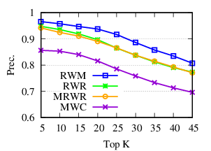
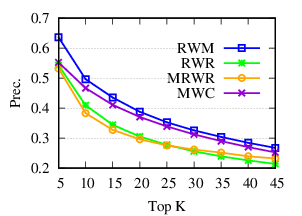
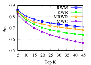
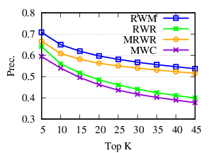
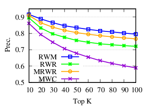
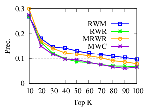
Ranking evaluation. To gain further insight into why RWM outperforms others, we compare RWM with other random walk based methods, i.e., RWR, MWC, and MRWR, as follows. Intuitively, nodes in the target local community should be assigned with high proximity scores w.r.t. the query node. Then we check the precision of top-ranked nodes based on score vectors of those models, i.e., prec. = (|top-𝑘 nodes ∩ ground truth|)/𝑘
(a)
RM |
(b)
BrainNet
|
(c)
6-NG
|
(d)
9-NG
|
(e)
Citeseer
|
(f)
DBLP
|
The precision results are shown in Fig. 3. First, we can see that precision scores of the selected methods decrease when the size of detected community 𝑘 increases. Second, our method consistently outperforms other random walk-based methods. Results indicate that RWM ranks nodes in the ground truth more accurately. Since ranking is the basis of a random walk based method for local community detection, better node-ranking generated by RWM leads to high-quality communities (Table 3).
6.3 Efficiency Evaluation. Note that the running time of RWM using basic power-iteration (Algorithm 1) is similar to the iteration-based random walk local community detection methods but RWM obtains better performance than other baselines with a large margin (Table 3). Thus, in this section, we focus on RWM and use synthetic datasets to evaluate its efficiency. There are three methods to update visiting probabilities in RWM: (1) power iteration method in Algorithm 1 (PowerIte), (2) power iteration with early stopping introduced in Sec. 5.1 (A1), and (3) partial updating in Sec. 5.2 (A2).

(a)
Total
time
w.r.t.
# of
networks |

(b)
Total
time
w.r.t.
# of
nodes |
We first evaluate the running time w.r.t. the number of networks. We generate 9 datasets with different numbers of networks (2 to 10). For each dataset, we first use a graph generator [16] to generate a base network consisting of 1,000 nodes and about 7,000 edges. Then we obtain multiple networks from the base network. In each network, we randomly delete 50% edges from the base network. For each dataset, we randomly select a node as the query and detect local communities. In Fig. 4(a), we report the running time of the three methods averaged over 100 trials. The early stopping in A1 saves time by about 2 times for the iteration method. The partial updating in A2 can further speed up by about 20 times. Furthermore, we can observe that the running time of A2 grows slower than PowerIte. Thus the efficiency gain tends to be larger with more networks.
Next, we evaluate the running time w.r.t. the number of nodes. Similar to the aforementioned generating process, we synthesize 4 datasets from 4 base networks with the number of nodes ranging from 104 to 107. The average node degree is 7 in each base network. For each dataset, we generate multiplex networks with three networks, by randomly removing half of the edges from the base network. The running time is shown in Fig. 4(b). Comparing to the power iteration method, the approximation methods are much faster, especially when the number of nodes is large. In addition, they grow much slower, which enables their scalability on even larger datasets.
We further check the number of visited nodes, which have positive
visiting probability scores in RWM, in different sized networks. In
Table 4, we show the number of visited nodes both at the splitting time
𝑇𝑒 and the end of updating (averaged over 100 trails). Note that
we compute 𝑇𝑒 = ⌈log λ  ⌉ according to Theorem 4 with
𝐾= 3,ϵ= 0.01,λ= 0.7. We see that in the end, only a very small
proportion of nodes are visited (for the biggest 107 network,
probability only propagates to 0.02% nodes). This demonstrates the
locality of RWM. Besides, in the first phase (early stop at 𝑇𝑒 ), visiting
probabilities are restricted in about 50 nodes around the query
node.
⌉ according to Theorem 4 with
𝐾= 3,ϵ= 0.01,λ= 0.7. We see that in the end, only a very small
proportion of nodes are visited (for the biggest 107 network,
probability only propagates to 0.02% nodes). This demonstrates the
locality of RWM. Besides, in the first phase (early stop at 𝑇𝑒 ), visiting
probabilities are restricted in about 50 nodes around the query
node.
| 104 | 105 | 106 | 107 | |
| # visited nodes (𝑇𝑒 ) | 47.07 | 50.58 | 53.27 | 53.54 |
| # visited nodes (end) | 1977.64 | 2103.43 | 2125.54 | 2177.70 |
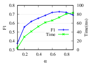
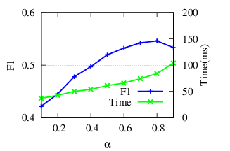
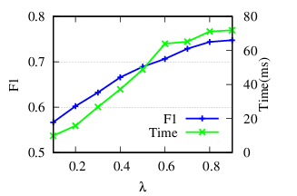
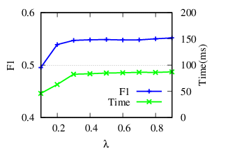
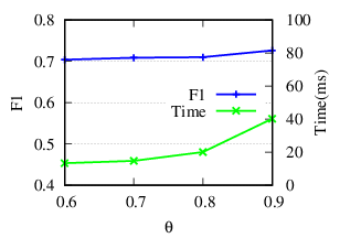
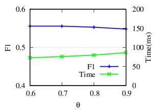
6.4 Parameter Study. In this section, we show the effects of the four important parameters in RWM: the restart factor α, the decay factor λ, tolerance ϵ for early stopping, and the covering factor θ in the partial updating. We report the F1 scores and running time on two representative datasets RM and 6-NG. Note that ϵ and θ control the trade-off between running time and accuracy. The parameter α controls the restart of a random walker in Eq. (5). The F1 scores and the running time w.r.t. α are shown in Fig. 5(a) and Fig. 5(b). When α is small, the accuracy increases as α increases because larger α encourages further exploration. When α reaches an optimal value, the accuracy begins to drop slightly. Because a too large α impairs the locality property of the restart strategy. The running time increases when α increases because larger α requires more iterations for score vectors to converge.
λ controls the updating of the relevance weights in Eq. (6). Results in Fig. 5(c) and Fig. 5(d) reflect that for RM, RWM achieves the best result when λ= 0.9. This is because large λ ensures that a enough number of neighbors are included when calculating relevance similarities. For 6-NG, RWM achieves high accuracy in a wide range of λ. For the running time, according to Theorem 4, larger λ results in larger 𝑇𝑒 , i.e., more iterations in the first phase, and longer running time.
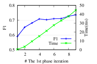
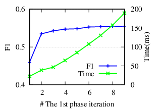
ϵ controls 𝑇𝑒 , the splitting time in the first phase. Instead of adjusting ϵ, we directly tune 𝑇𝑒 . Theoretically, a larger 𝑇𝑒 (i.e., a smaller ϵ) leads to more accurate results. Based on results shown in Fig. 5(e) and Fig. 5(f), we notice that RWM achieves good performance even with a small 𝑇𝑒 in the first phase. The running time decreases significantly as well. This demonstrates the rationality of early stopping.
θ controls the number of updated nodes (in Sec. 5.2). In Fig. 5(g) and 5(h), we see that the running time decreases along with θ decreasing, because less number of nodes are updated. The consistent accuracy performance shows the effectiveness of the speeding-up strategy.
(a)
RM |
(b)
6-NG
|
(c)
RM |
(d)
6-NG
|
(e)
RM |
(f)
6-NG
|
(g)
RM |
(h)
6-NG
|
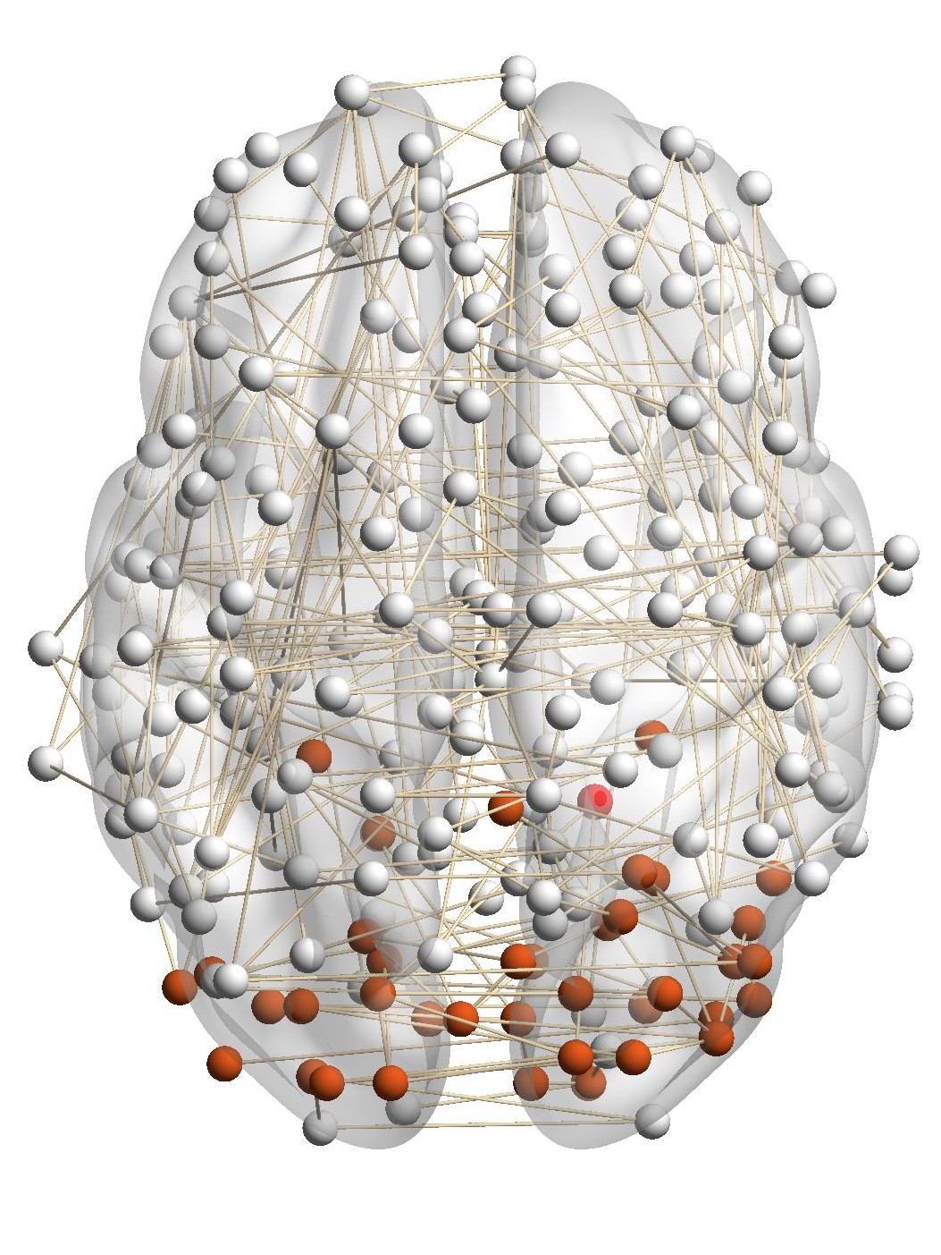
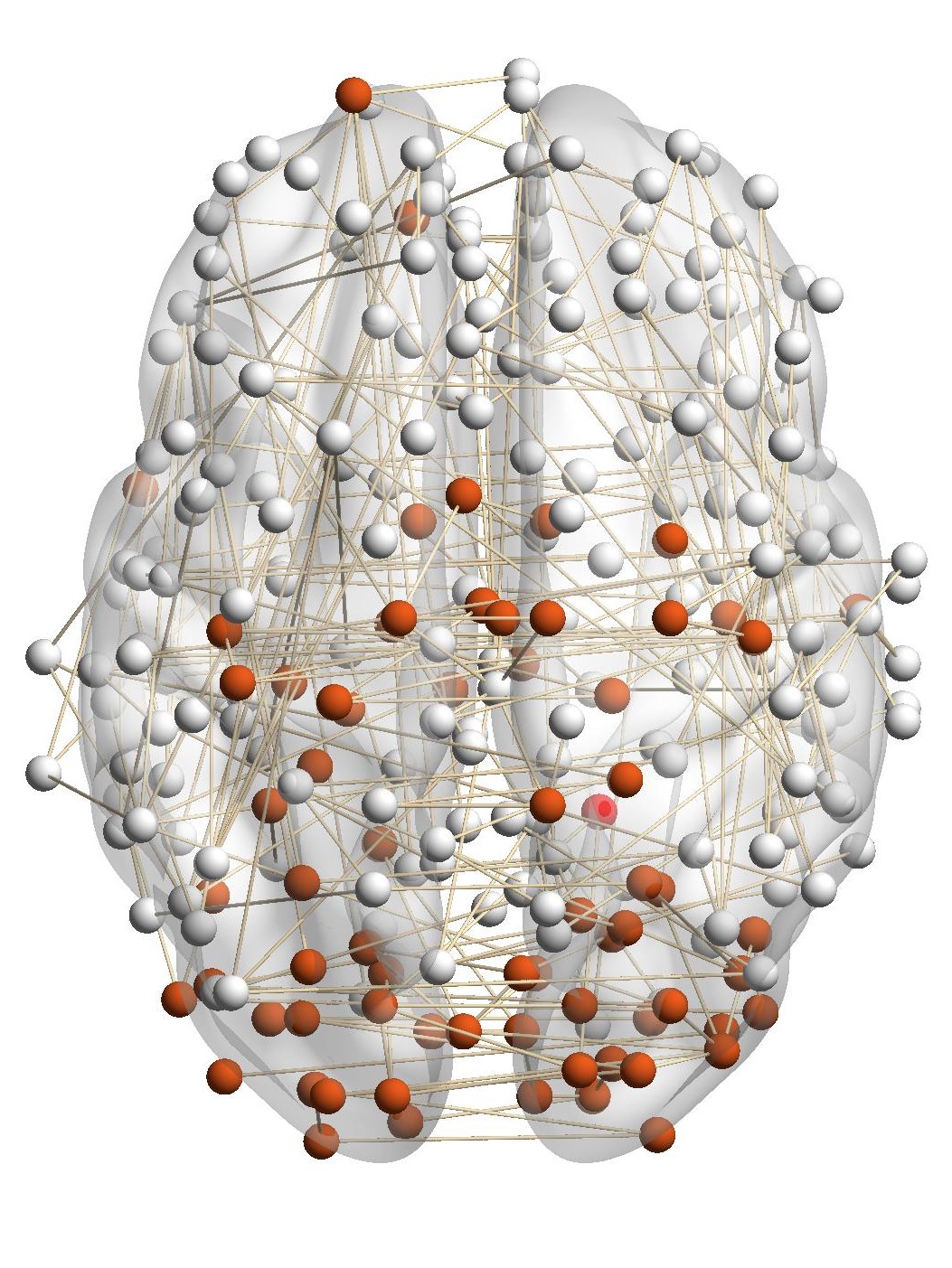
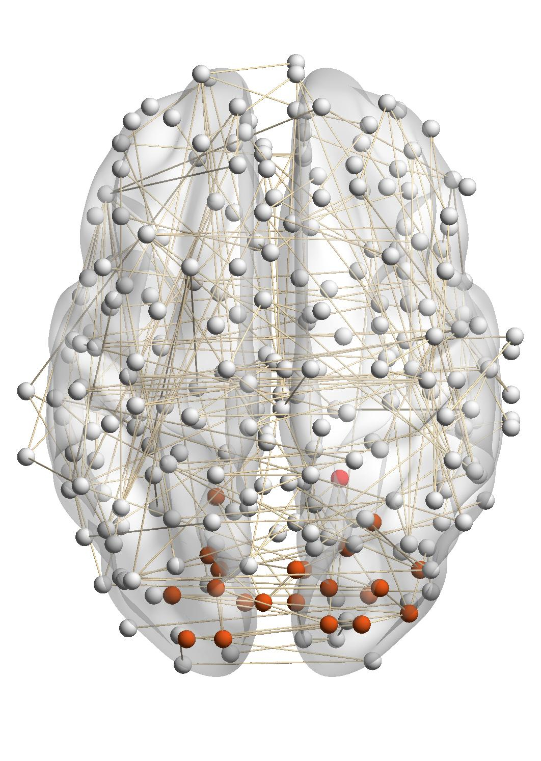
6.5 Case Studies. BrainNet and DBLP are two representative datasets for multiplex networks (with the same node set) and the general multi-domain network (with flexible nodes and edges). We do two case studies to show the detected local communities by RWM. Case Study on the BrainNet Dataset. Detecting and monitoring functional systems in the human brain is an important task in neuroscience. Brain networks can be built from neuroimages where nodes and edges are brain regions and their functional relations. In many cases, however, the brain network generated from a single subject can be noisy and incomplete. Using brain networks from many subjects helps to identify functional systems more accurately. For example, brain networks from three subjects are shown in Fig. 6. Subjects 1 and 2 have similar visual conditions (red nodes); subjects 1 and 3 are with similar auditory conditions (blue nodes). For a given query region, we want to find related regions with the same functionality.
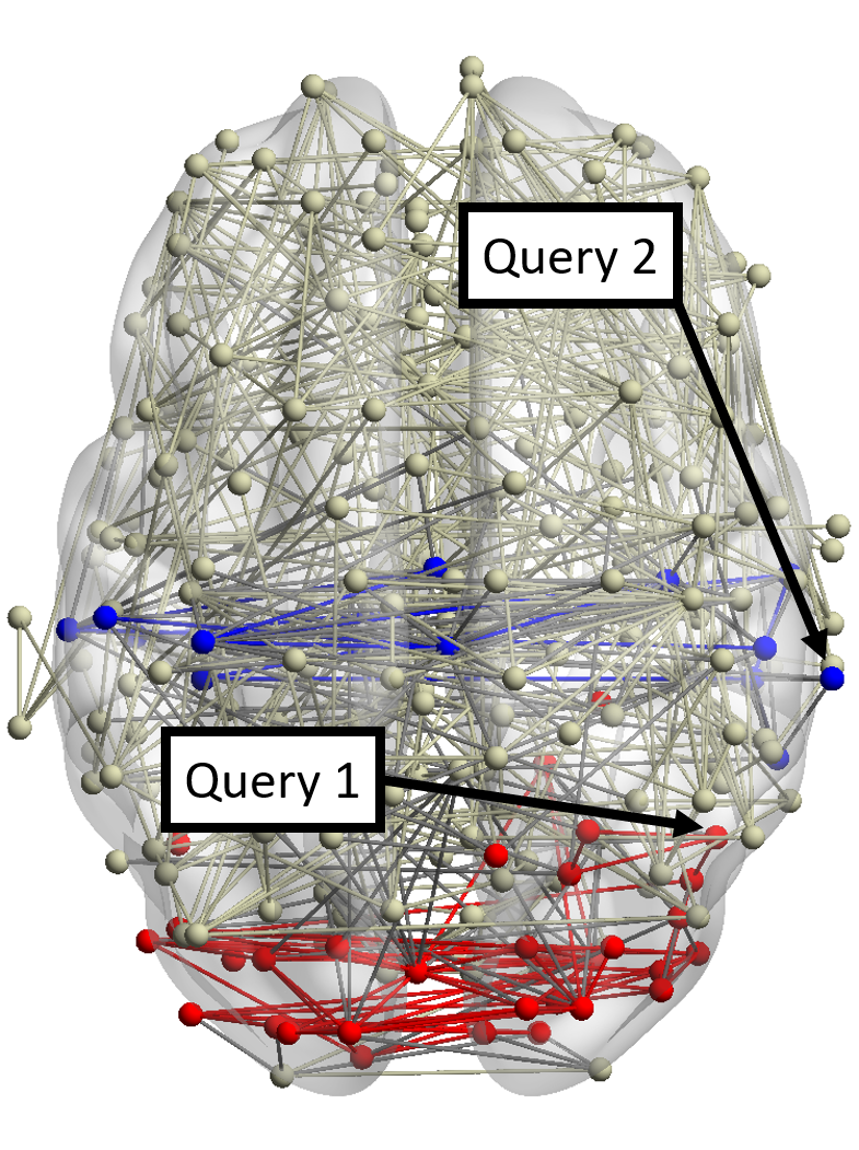
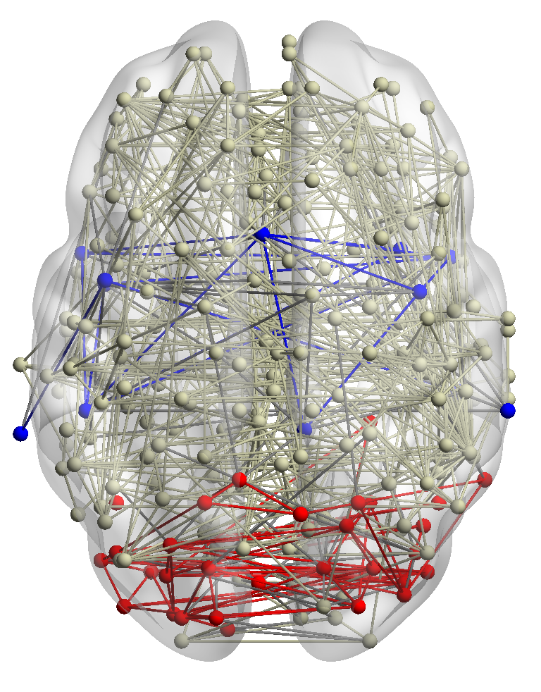
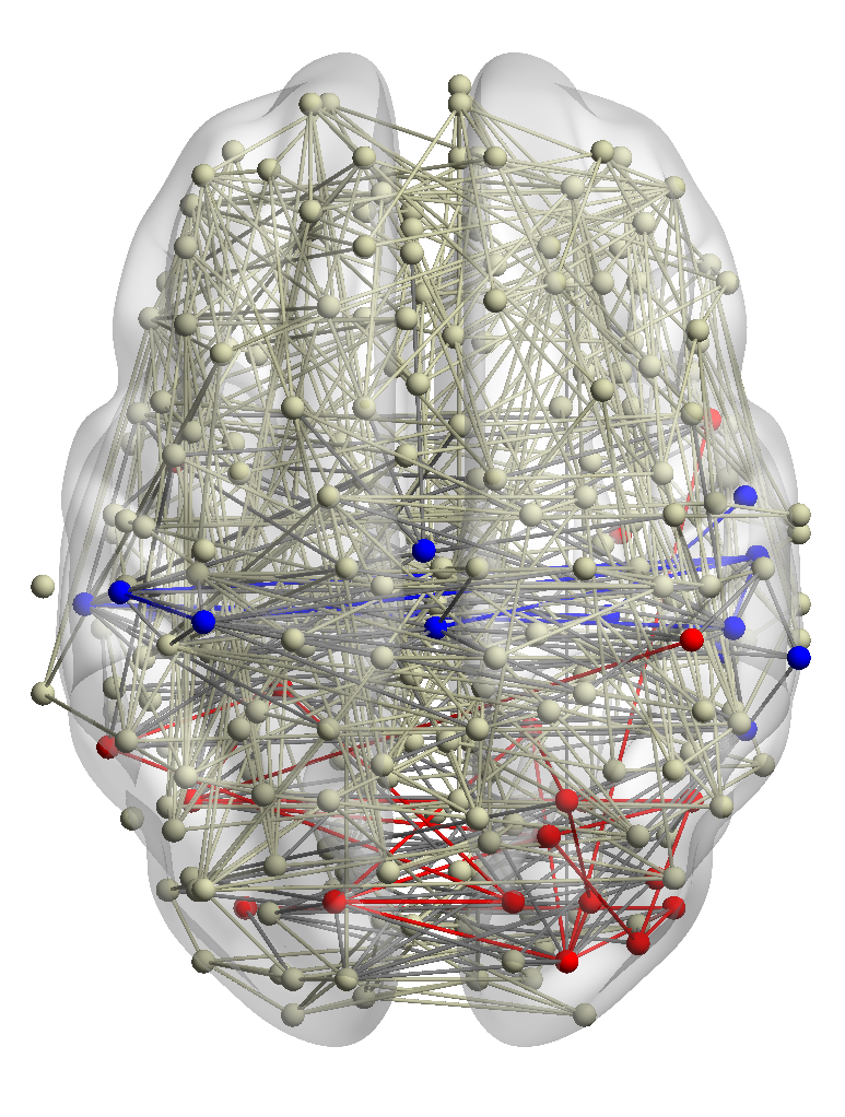
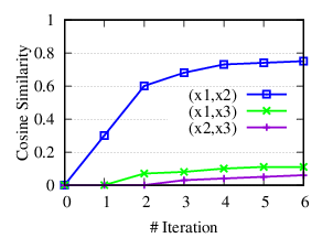
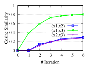
•Detect relevant networks. To see whether RWM can automatically detect relevant networks, we run RWM model for Query 1 and Query 2 in Fig. 6 separately. Fig. 7 shows the cosine similarity between the visiting probability vectors of different walkers along iterations. x1, x2, and x3 are the three visiting vectors on the three brain networks, respectively. We see that the similarity between the visiting histories of walkers in relevant networks, i.e., subjects 1 and 2 in Fig. 7(a), subjects 1 and 3 in 7(b), increases along with the updating. But similarities in query-oriented irrelevant networks are very low during the whole process. This indicates that RWM can actively select query-oriented relevant networks to help better capture the local structure for each network.
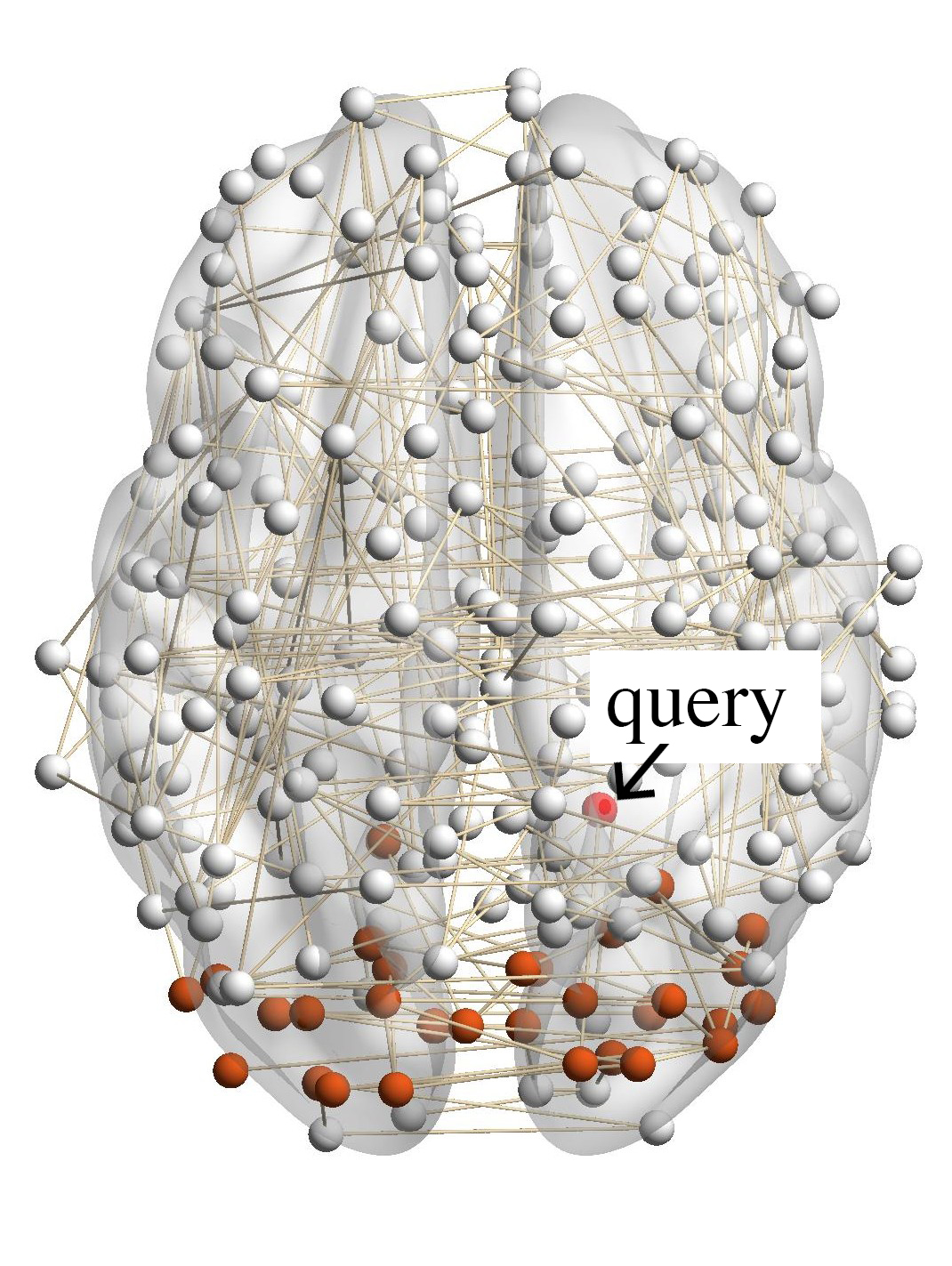
•Identify functional systems. In this case study, we further evaluate the detected results of RWM in the BrainNet dataset with the other two methods. Note that MRWR and ML-LCD can only find a query-oriented local community in the network containing the query node.
Fig. 8(a) shows a brain network of a subject with a given query node and its ground truth local community (red nodes). We run the three methods aggregating information from all other brain networks in the dataset. The identified communities are highlighted in red in Fig. 8. It’s shown that the community detected by our method is very similar to the ground truth. MRWR (Fig. 8(b)) includes many false-positive nodes. The reason is that MRWR assumes all networks are similar and treat them equally. While ML-LCD (Fig. 8(d)) neglects some nodes in the boundary region.
(a)
Groud
Truth |
(b)
RWM
(ours) |
(c)
MRWR |
(d)
ML-LCD |
Case Study on DBLP Dataset. In the general multiple networks, for a query node from one network, we only have the ground truth local community in that network but no ground truth about the relevant local communities in other networks. So in this section, we use DBLP as a case study to demonstrate the relevance of local communities detected from other networks by RWM. We use Prof. Danai Koutra from UMich as the query. The DBLP dataset was collected in May 2014 when she was a Ph.D. student advised by Prof. Christos Faloutsos. Table 5 shows the detected author community and paper community. Due to the space limitation, instead of showing the details of the paper community, we list venues that these papers published in. For example, “KDD(3)” means that 3 KDD papers are included in the detected paper community. The table shows that our method can detect local communities from both networks with high qualities. Specifically, the detected authors are mainly from her advisor’s group. The detected paper communities are mainly published in Database/Data Mining conferences.
| Author community | Paper community |
| Danai Koutra (query) | KDD (3) |
| Christos Faloutsos | PKDD (3) |
| Evangelos Papalexakis | PAKDD (3) |
| U Kang | SIGMOD (2) |
| Tina Eliassi-Rad | ICDM (2) |
| Michele Berlingerio | TKDE(1) |
| Duen Horng Chau | ICDE (1) |
| Leman Akoglu | TKDD (1) |
| Jure Leskovec | ASONAM (1) |
| Hanghang Tong | WWW(1) |
| ... | ... |
7 Conclusion
In this paper, we propose a novel random walk model, RWM, for local community detection in multiple networks. Unlike other baselines, RWM can detect all query-relevant local communities from all networks. Random walkers in different networks sent by RWM mutually affect their visiting probabilities in a reinforced manner. By aggregating their effects from query-relevant local subgraphs in different networks, RWM restricts walkers’ most visiting probabilities near the query nodes. Rigorous theoretical foundations are provided to verify the effectiveness of RWM. Two speeding-up strategies are also developed for efficient computation. Extensive experimental results verify the advantages of RWM in effectiveness and efficiency.
ACKNOWLEDGMENTS
This project was partially supported by NSF projects IIS-1707548 and CBET-1638320.
[1] Morteza Alamgir and Ulrike Von Luxburg. 2010. Multi-agent random walks for local clustering on graphs. In ICDM. 18–27.
[2] Reid Andersen, Fan Chung, and Kevin Lang. 2006. Local graph partitioning using pagerank vectors. In FOCS. 475–486.
[3] Nicola Barbieri, Francesco Bonchi, Edoardo Galimberti, and Francesco Gullo. 2015. Efficient and effective community search. Data mining and knowledge discovery 29, 5 (2015), 1406–1433.
[4] Yuchen Bian, Dongsheng Luo, Yaowei Yan, Wei Cheng, Wei Wang, and Xiang Zhang. 2019. Memory-based random walk for multi-query local community detection. Knowledge and Information Systems (2019), 1–35.
[5] Yuchen Bian, Jingchao Ni, Wei Cheng, and Xiang Zhang. 2017. Many heads are better than one: Local community detection by the multi-walker chain. In ICDM. 21–30.
[6] Yuchen Bian, Jingchao Ni, Wei Cheng, and Xiang Zhang. 2019. The multi-walker chain and its application in local community detection. Knowledge and Information Systems 60, 3 (2019), 1663–1691.
[7] Yuchen Bian, Yaowei Yan, Wei Cheng, Wei Wang, Dongsheng Luo, and Xiang Zhang. 2018. On multi-query local community detection. In ICDM. 9–18.
[8] Manlio De Domenico, Andrea Lancichinetti, Alex Arenas, and Martin Rosvall. 2015. Identifying modular flows on multilayer networks reveals highly overlapping organization in interconnected systems. Physical Review X 5, 1 (2015), 011027.
[9] Xin Huang, Hong Cheng, Lu Qin, Wentao Tian, and Jeffrey Xu Yu. 2014. Querying k-truss community in large and dynamic graphs. In SIGMOD. 1311–1322.
[10] Xin Huang, Laks VS Lakshmanan, and Jianliang Xu. 2019. Community Search over Big Graphs. Synthesis Lectures on Data Management 14, 6 (2019), 1–206.
[11] Xin Huang, Laks VS Lakshmanan, Jeffrey Xu Yu, and Hong Cheng. 2015. Approximate closest community search in networks. PVLDB 9, 4 (2015), 276–287.
[12] Roberto Interdonato, Andrea Tagarelli, Dino Ienco, Arnaud Sallaberry, and Pascal Poncelet. 2017. Local community detection in multilayer networks. Data Mining and Knowledge Discovery 31, 5 (2017), 1444–1479.
[13] Jungeun Kim and Jae-Gil Lee. 2015. Community detection in multi-layer graphs: A survey. ACM SIGMOD Record 44, 3 (2015), 37–48.
[14] Mikko Kivelä, Alex Arenas, Marc Barthelemy, James P Gleeson, Yamir Moreno, and Mason A Porter. 2014. Multilayer networks. Journal of complex networks 2, 3 (2014), 203–271.
[15] Kyle Kloster and David F Gleich. 2014. Heat kernel based community detection. In SIGKDD. 1386–1395.
[16] Andrea Lancichinetti and Santo Fortunato. 2009. Benchmarks for testing community detection algorithms on directed and weighted graphs with overlapping communities. Physical Review E (2009).
[17] Yixuan Li, Kun He, David Bindel, and John E Hopcroft. 2015. Uncovering the small community structure in large networks: A local spectral approach. In WWW. 658–668.
[18] Kar Wai Lim and Wray Buntine. 2016. Bibliographic analysis on research publications using authors, categorical labels and the citation network. Machine Learning 103, 2 (2016), 185–213.
[19] Daqian Lu and Hao Zhang. 1986. Stochastic process and applications. Tsinghua University Press.
[20] Dongsheng Luo, Jingchao Ni, Suhang Wang, Yuchen Bian, Xiong Yu, and Xiang Zhang. 2020. Deep Multi-Graph Clustering via Attentive Cross-Graph Association. In WSDM. 393–401.
[21] Peter J Mucha, Thomas Richardson, Kevin Macon, Mason A Porter, and Jukka-Pekka Onnela. 2010. Community structure in time-dependent, multiscale, and multiplex networks. Science 328, 5980 (2010), 876–878.
[22] Jingchao Ni, Shiyu Chang, Xiao Liu, Wei Cheng, Haifeng Chen, Dongkuan Xu, and Xiang Zhang. 2018. Co-regularized deep multi-network embedding. In WWW. 469–478.
[23] Satu Elisa Schaeffer. 2005. Stochastic local clustering for massive graphs. In PAKDD. 354–360.
[24] Jing Shan, Derong Shen, Tiezheng Nie, Yue Kou, and Ge Yu. 2016. Searching overlapping communities for group query. World Wide Web 19, 6 (2016), 1179–1202.
[25] Jie Tang, Jing Zhang, Limin Yao, Juanzi Li, Li Zhang, and Zhong Su. 2008. Arnetminer: extraction and mining of academic social networks. In SIGKDD. 990–998.
[26] Hanghang Tong, Christos Faloutsos, and Jia-Yu Pan. 2006. Fast random walk with restart and its applications. In ICDM. 613–622.
[27] David C Van Essen, Stephen M Smith, Deanna M Barch, Timothy EJ Behrens, Essa Yacoub, Kamil Ugurbil, Wu-Minn HCP Consortium, et al. 2013. The WU-Minn human connectome project: an overview. Neuroimage 80 (2013), 62–79.
[28] Twan Van Laarhoven and Elena Marchiori. 2016. Local network community detection with continuous optimization of conductance and weighted kernel k-means. The Journal of Machine Learning Research 17, 1 (2016), 5148–5175.
[29] Nate Veldt, Christine Klymko, and David F Gleich. 2019. Flow-based local graph clustering with better seed set inclusion. In SDM. 378–386.
[30] Yubao Wu, Yuchen Bian, and Xiang Zhang. 2016. Remember where you came from: on the second-order random walk based proximity measures. Proceedings of the VLDB Endowment 10, 1 (2016), 13–24.
[31] Yubao Wu, Ruoming Jin, Jing Li, and Xiang Zhang. 2015. Robust local community detection: on free rider effect and its elimination. PVLDB 8, 7 (2015), 798–809.
[32] Yubao Wu, Xiang Zhang, Yuchen Bian, Zhipeng Cai, Xiang Lian, Xueting Liao, and Fengpan Zhao. 2018. Second-order random walk-based proximity measures in graph analysis: formulations and algorithms. The VLDB Journal 27, 1 (2018), 127–152.
[33] Yaowei Yan, Yuchen Bian, Dongsheng Luo, Dongwon Lee, and Xiang Zhang. 2019. Constrained Local Graph Clustering by Colored Random Walk. In WWW. 2137–2146.
[34] Yaowei Yan, Dongsheng Luo, Jingchao Ni, Hongliang Fei, Wei Fan, Xiong Yu, John Yen, and Xiang Zhang. 2018. Local Graph Clustering by Multi-network Random Walk with Restart. In PAKDD. 490–501.
[35] Hao Yin, Austin R Benson, Jure Leskovec, and David F Gleich. 2017. Local higher-order graph clustering. In SIGKDD. 555–564.
[36] Long Yuan, Lu Qin, Wenjie Zhang, Lijun Chang, and Jianye Yang. 2017. Index-based densest clique percolation community search in networks. IEEE Transactions on Knowledge and Data Engineering 30, 5 (2017), 922–935.