Towards Inductive and Efficient Explanations for Graph Neural Networks
Dongsheng Luo, Tianxiang Zhao, Wei Cheng, Dongkuan Xu, Feng Han, Wenchao Yu, Xiao Liu,
Haifeng Chen, Xiang Zhang
Abstract
Despite recent progress in Graph Neural Networks (GNNs), explaining predictions made by GNNs remains a challenging
and nascent problem. The leading method mainly considers the local explanations, i.e., important subgraph structure and
node features, to interpret why a GNN model makes the prediction for a single instance, e.g. a node or a graph. As a
result, the explanation generated is painstakingly customized at the instance level. The unique explanation interpreting each
instance independently is not sufficient to provide a global understanding of the learned GNN model, leading to the lack of
generalizability and hindering it from being used in the inductive setting. Besides, training the explanation model explaining
for each instance is time-consuming for large-scale real-life datasets. In this study, we address these key challenges and
propose PGExplainer, a parameterized explainer for GNNs. PGExplainer adopts a deep neural network to parameterize the
generation process of explanations, which renders PGExplainer a natural approach to multi-instance explanations. Compared
to the existing work, PGExplainer has better generalization ability and can be utilized in an inductive setting without training
the model for new instances. Thus, PGExplainer is much more efficient than the leading method with significant speed-up. In
addition, the explanation networks can also be utilized as a regularizer to improve the generalization power of existing GNNs
when jointly trained with downstream tasks. Experiments on both synthetic and real-life datasets show highly competitive
performance with up to 24.7% relative improvement in AUC on explaining graph classification over the leading baseline.
Index Terms
Graph neural networks, Deep learning, Interpretability
∙ D. Luo is with Florida International University
E-mail: dluo@fiu.edu
∙ T. Zhao, X. Liu, and X. Zhang are with the Pennsylvania State University, State College, PA 16802.
E-mail: {tkz5084, xxl213, xzz89}@psu.edu.
∙ W. Cheng, W. Yu, and H. Cheng are with NEC Lab America, Inc.
E-mail: {weicheng, wyu,haifeng}@nec-labs.com
∙ D. Xu is with North Carolina State University
E-mail: dxu27@ncsu.edu
∙ F. Han is with the University of California, Berkeley.
E-mail: feng.han@berkeley.edu.
1 Introduction
Graph Neural Networks (GNNs) are powerful tools for representation learning of graph-structured data, such as social
networks [54], document citation graphs [44], and microbiological graphs [52]. GNNs routinely adopt a message passing scheme to
learn node representations by aggregating representation vectors of their neighbors [55, 17]. This scheme enables GNN to capture
both node features and graph topology. GNN-based methods have achieved state-of-the-art performance in node classification,
graph classification, and link prediction [23, 53, 63].
Despite their remarkable effectiveness, the rationales of predictions made by GNNs are not easy for humans to understand. Since
GNNs aggregate both node features and graph topology to make predictions, to understand predictions made by GNNs, important
subgraphs and/or a set of features, which are also known as explanations, need to be uncovered. In the literature, although a variety
of efforts have been undertaken to interpret general deep neural networks, existing approaches [6, 33, 14, 37, 50, 21, 22] in this
line fall short in their ability to explain graph structures, which is essential for GNNs. Explaining predictions made
by GNNs remains a challenging problem, on which few methods have been proposed [58, 48, 62, 60, 61]. The
combinatorial nature of explaining graph structures makes it difficult to design models that are both robust and
efficient.
Recently, the first general model-agnostic approach for GNNs, GNNExplainer [58], was proposed to address the problem. It
takes a trained GNN and its predictions as inputs to provide interpretable explanations for a given instance, e.g. a node or a graph.
The explanation includes a compact subgraph structure and a small subset of node features that are crucial in GNN’s prediction for
the target instance. Nevertheless, there are several limitations to the existing approach. First, GNNExplainer largely focuses on
providing the local interpretability by generating a painstakingly customized explanation for a single instance individually and
independently. The explanation provided by GNNExplainer is limited to a single instance, making GNNExplainer difficult to be
applied in the inductive setting because the explanations are hard to generalize to other unexplained nodes. As
pointed out in previous studies, models interpreting each instance independently are not sufficient to provide a
global understanding of the trained model [21]. Furthermore, GNNExplainer has to be retrained for every single
explanation. As a result, in real-life scenarios where plenty of nodes need to be interpreted, GNNExplainer would be
time-consuming and impractical. Moreover, as GNNExplainer was developed for interpreting individual instances,
the authors further provided additional ad-hoc post-analysis, such as identifying the representative instance and
graph alignment, to extract the shared motifs to explain a set of instances (e.g., graphs of a given class in graph
classification task) [58]. Since the explanatory motifs are not learned end-to-end, the model however may suffer from
suboptimal generalization performance. How to explain predictions of GNNs on a set of instances collectively and easily
generalize the learned explainer model to other instances in the inductive setting remains largely unexplored in the
literature.
To provide a global understanding of predictions made by GNNs, in this study, we emphasize the collective and inductive nature
of this problem that an explanation model should be able to explain a set of instances and infer new instances without re-training.
We present an inductive and effective explanation model to interpret graph neural networks, denoted by PGExplainer (Figure 1).
PGExplainer is a general explainer that applies to any GNN based models for various tasks, including node classification, graph
classification, and link prediction. Specifically, a generative probabilistic model for graph data is utilized in PGExplainer. Generative
models have shown the power to learn succinct underlying structures from the observed graph data [27]. PGExplainer
uncovers these underlying structures as the explanations, which is believed to make the most contribution to GNNs’
predictions [41]. We model the underlying structure as edge distributions, where the explanatory graph is sampled from. To
collectively explain predictions of multiple instances, the generation process in PGExplainer is parameterized with a
deep neural network. Since the neural network parameters are shared across the population of explained instances,
PGExplainer is naturally applicable to provide global explanations of GNNs. Furthermore, PGExplainer has better
generalization power because a trained PGExplainer model can be utilized in an inductive setting to infer explanations of
unexplained nodes without retraining the explanation model. This also makes PGExplainer much faster than the existing
work.
Another application of PGExplainer is to learn graph structures for GNN models, which are error-prone to noisy topological
structures. GNNs learn node embeddings by recursively aggregating messages from their neighborhoods. Such message passing
mechanism is associated with cascading effects that small noise may propagate to neighboring nodes and leads to sub-optimal
representations of many others. To improve the robustness of GNN models, graph structure learning methods first learn a
denoised graph structure for the downstream task [67]. However, the original input graph is insufficiently analyzed in
existing state-of-the-art methods since they will be dropped once the subgraphs are extracted [39, 66]. Based upon
PGExplainer, we propose a more flexible method to learn compact subgraph structures that maximizes the mutual
information between the subgraph and labels in the downstream task. When the downstream task objective is jointed
optimized with a size constraint regularizer, our method can improve the accuracy performance and robustness of
GNNs.
Experimental results on both synthetic and real-life datasets demonstrate that PGExplainer can achieve consistent and accurate
explanations, bringing up to 24.7% improvement in AUC over the SOTA method on explaining graph classification with significant
speed-up.
2 Related work
Graph neural networks. Graph Neural networks (GNNs) have achieved remarkable success in various tasks, including node
classification [31, 23, 53], graph classification [12], and link prediction [63]. The study of GNNs was initiated in [19], and then
extended in [47]. These methods iteratively aggregate neighbor information to learn node representations until reaching a static
state. Inspired by the success of convolutional neural networks (CNNs) in computer vision, attempts of applying convolutional
operations to graphs were derived based on graph spectral theory [4] and graph Fourier transformation [49]. In recent work, GNNs
broadly encode node features as messages and adopt the message passing mechanism to propagate and aggregate them along
edges to learn node/graph representations, which are then utilized for downstream tasks [31, 12, 47, 36, 53, 40].
For efficiency consideration, localized filters were proposed to reduce computation cost [23]. The self-attention
mechanism was introduced to GNNs in GAT to differentiate the importance of neighbors [53]. Xu. et al. analyzed the
relationship between GNNs and Weisfeiler-Lehman graph isomorphism test, and showed the express power of
GNNs [55].
Explaining GNNs. Interpretability and feature selection have been extensively addressed in neural networks. Methods demystifying
complicated deep learning models can be grouped into two main families, whitebox and blackbox [21, 22]. Whitebox mechanisms
mainly focus on yielding explanations for individual predictions. Forward and backward propagation based methods are used
routinely in whitebox mechanisms. Forward propagation based methods broadly perturb the input and/or hidden representations
and check the corresponding updating results in the downstream task [10, 15, 35]. The underlying intuition is that the outputs of
the downstream task are likely to significantly change if important features are occluded. Backward propagation
based methods, in general, infer important features from the gradients of the deep neural networks. They compute
weights of features by propagating the gradients from the output back to the input. Blackbox methods generate
explanations by locally learning interpretable models, such as linear models, and additive models to approximate the
predictions [38, 5, 64, 65].
Following the line of forward propagation methods, GNNExplainer initiates the research on explaining predictions on
graph-structured data [58]. It excludes certain edges and node features to observe the changes in node/graph classification.
Explanations (subgraphs/important features) are extracted by maximizing the mutual information between the distribution of
possible subgraphs and the GNN’s prediction. However, similar to other forward propagation methods, GNNExplainer generates
customized explanations for single instance prediction independently, making it insufficient to provide a global understanding of
the trained GNN model. Besides, it is naturally difficult to be applied in the inductive setting and provide explanations for multiple
instances.
Graph generation. PGExplainer learns a probabilistic graph generative model to provide explanations for GNNs.
The first model generating random graph is the Erdős–Rényi model [16, 13]. In the random graph proposed by
Gilbert, each potential edge is independently chosen from a Bernoulli distribution. Some works generate graphs with
certain properties reflected, such as pairwise distances betweenness [7], node degree distribution [34], and spectral
properties [26, 2]. In recent years, deep learning models have shown great potential to generate graphs with complex properties
preserved [59, 20, 41]. However, these methods mainly aim to generate graphs that reflect certain properties in the training
graphs.
3 Background
We first describe notations, and then provide some background on graph neural networks.
Notations. Let G = ( ,
, ) represent the graph with = {v1,v2...vN} denoting the node set and ∈× as the edge set. The
numbers of nodes and edges are denoted by N and M, respectively. A graph can be described by an adjacency matrix
A ∈{0,1}N×N, with aij = 1 if there is an edge connecting node i and j, and aij = 0 otherwise. Nodes in are associated with the
d-dimensional features, denoted by X ∈ℝN×d.
) represent the graph with = {v1,v2...vN} denoting the node set and ∈× as the edge set. The
numbers of nodes and edges are denoted by N and M, respectively. A graph can be described by an adjacency matrix
A ∈{0,1}N×N, with aij = 1 if there is an edge connecting node i and j, and aij = 0 otherwise. Nodes in are associated with the
d-dimensional features, denoted by X ∈ℝN×d.
Graph neural networks. GNNs adopt the message-passing mechanism to propagate and aggregate information along edges in the
input graph to learn node representations [31, 23, 53, 17]. Each GNN layer includes three essential steps. First, at the propagation
step of the i-th GNN layer, for each edge (i,j), GNN computes a message mijl = Message(hil-1,hjl-1), where hil-1 and hjl-1 are
representations of vi and vj in previous layer, respectively. Second, at the aggregation step, for each node vi, GNN aggregates
messages received from its neighbor nodes, denoted by  i, with an aggregation function mi⋅l = aggregation({mijl|j ∈i}). Last,
at the updating step, GNN updates the vector representation for each node vi via hil = update(mi⋅l,hil-1), a function taking the
aggregated message and the representation of itself as inputs. Hidden representation of the last GNN layer serve as the final node
representation: zi = hiL, which is then used for downstream tasks, such as node/graph classification, and link
prediction.
i, with an aggregation function mi⋅l = aggregation({mijl|j ∈i}). Last,
at the updating step, GNN updates the vector representation for each node vi via hil = update(mi⋅l,hil-1), a function taking the
aggregated message and the representation of itself as inputs. Hidden representation of the last GNN layer serve as the final node
representation: zi = hiL, which is then used for downstream tasks, such as node/graph classification, and link
prediction.
4 The PGExplainer
In this section, we introduce PGExplainer. Different from GNNExplainer which provides explanations on both structure and
features, PGExplainer focuses on explanation on graph structures because feature explanation in GNNs is similar to that in
non-graph neural networks, which has been extensively studied in the literature [1, 21, 38, 45, 10, 15, 35]. PGExplainer is flexible
and applicable to interpreting all kinds of GNNs. We start with the learning objective of PGExplainer (Section 4.1) and then present
the reparameterization strategy for efficient optimization (Section 4.2). In Section 4.3, we specify particular instantiations to
understand GNNs on node and graph classifications.
4.1 The learning objective
The literature has shown that real-life graphs are with underlying structures [41, 43]. To explain predictions made by a
GNN model, we divide the original input graph Go into two subgraphs: Go = Gs + ΔG, where Gs presents the
underlying subgraph that makes important contributions to GNN’s predictions, which is the expected explanatory
graph, and ΔG consists of the remaining task-irrelevant edges for predictions made by the GNN. Following [58],
PGExplainer finds Gs by maximizing the mutual information between the GNN’s predictions and the underlying structure
Gs:
where Y o is the prediction of the GNN model with Go as the input. The mutual information quantifies the probability of prediction
Y o when the input graph to the GNN model is limited to the explanatory graph Gs. The intuition behind this comes from the
traditional forward propagation-based methods for the white box explanation [10]. For example, if removing an edge (i,j)
dramatically changes the prediction in the GNN, then this edge is important and should be included in Gs. Otherwise, it can be
considered as irrelevant edge for the GNN model to make the prediction. Since H(Y o) is only related to the GNN model whose
parameters are fixed in the explanation stage, the objective is equivalent to minimizing the conditional entropy
H(Y o|G = Gs).
However, the direct optimization of the above objective function is intractable as there are 2M candidates for
Gs. Thus, we consider a relaxation by assuming that the explanatory graph is a Gilbert random graph [16], where
selections of edges from the original input graph Go are conditionally independent to each other. Let eij ∈× be the
binary variable indicating whether the edge is selected, with eij = 1 if the edge (i,j) is selected, and 0 otherwise. Let
G be the random graph variable. Based on the above assumption, the probability of a graph G can be factorized
as:
A straightforward instantiation of P(eij) is the Bernoulli distribution eij ~ Bern(θij). P(eij = 1) = θij is the probability that edge
(i,j) exists in G. With this relaxation, we thus can rewrite the objective as:
where q(Θ) is the distribution of the explanatory graph parameterized by θ’s.
4.2 The reparameterization trick
Due to the discrete nature of Gs, we relax edge weights from binary variables to continuous variables in the range (0,1) and
adopt the reparameterization trick to efficiently optimize the objective function with gradient-based methods [29]. We approximate
the sampling process Gs ~ q(Θ) with a determinant function of parameters Ω, temperature τ, and an independent random
variable ϵ: Gs ≈Ĝs = fΩ(Go,τ,ϵ). The temperature τ is used to control the approximation. Here we utilize the binary
concrete distribution as the instantiation [42]. Specifically, the weight êij ∈ (0,1) of edge (i,j) in Ĝs is calculated
by:
where σ(⋅)is the Sigmoid function, and ωij ∈ℝ is the parameter. When τ → 0, the weight êij is binarized with
limτ→0P(êij = 1) =  . Since P(eij = 1) = θij, by choosing ωij = log
  , we have limτ→0Ĝs = Gs. This demonstrates
the rationality of using binary concrete distribution to approximate the Bernoulli distribution. Moreover, with temperature τ > 0,
the objective function is smoothed with a well-defined gradient
, we have limτ→0Ĝs = Gs. This demonstrates
the rationality of using binary concrete distribution to approximate the Bernoulli distribution. Moreover, with temperature τ > 0,
the objective function is smoothed with a well-defined gradient  .Thus, with reparameterization, the objective in Eq. (3)
becomes:
.Thus, with reparameterization, the objective in Eq. (3)
becomes:
Considering efficient optimization, we follow [58] to modify the conditional entropy with cross-entropy H(Y o,Ŷs), where Ŷs is
the prediction of the GNN model with Ĝs as the input. With the above relaxations, we adopt Monte Carlo to approximately optimize
the objective function:
where Φ denotes the parameters in the trained GNN, K is the total number of sampled graph, C is the number of labels, Ĝs(k) is the
k-th sampled graph with Eq. (4), parameterized by Ω.
4.3 Explanation of graph neural networks with a global view
Although explanations provided by the leading method GNNExplainer [58] preserve the local fidelity, they do not help to
understand the general picture of the model across a population [56]. Furthermore, various GNN based models have been applied
to analyze graph data with millions of instances [57], the cost of applying local explanations one-by-one can be prohibitive with
such large datasets in practice. On the other hand, explanations with a global view of the model ascertain users’ trust [45].
Furthermore, these models can generalize explanations to new instances without retraining, making it more efficient to explain large
scale datasets.
To have a global view of a GNN model, our method collectively explains predictions made by a trained model on multiple
instances. Instead of treating Ω in Eq. (6) as independent variables, we utilize a parameterized network to learn to generate
explanations from the trained GNN model. After training, the parameterized network can be used in the inductive setting to
provide explanations for unexplained instances. In general, GNN based models first learn node representations and then feed the
vector representations to downstream tasks [23, 31, 53]. We denote these two functions by GNNEΦ0(⋅) and GNNCΦ1(⋅),
respectively. For GNNs without explicit classification layers, we use the last layer instead. As a result, we can represent a GNN
model with:
Z is the matrix of node representations encoding both features and structure of the input graph, which is used as an input in the
explanation network to calculate the parameter Ω:
Ψ denotes parameters in the explanation network, which is shared by all edges among the population. Therefore, PGExplainer can
be utilized to collectively provide explanations for multiple instances. Specifically, in the collective setting with instance set  , the
objective of PGExplainer is:
, the
objective of PGExplainer is:
where G(i) is the input graph and Ĝs(i,k) is the k-th sampled graph with Eq. (4 ,8) for i-th instance. We consider both graph and
node classifications and specify an instantiation for each task. Solutions for other tasks, such as link prediction, are similar and thus
omitted.
Explanation network for node classification. Considering that explanations for nodes in a graph may appear diverse
structures [58], especially for nodes with different labels. For example, an edge (i,j) is important for the prediction of node u, but
not for another node v. Based on this motivation, we implement the Ω = gΨ(Go,Z) to explain the prediction of node v
with:
MLPΨ is a multi-layer neural network parameterized with Ψ and [⋅;⋅] is the concatenation operation.
___________________________________________________________________________________________________
Algorithm 1: Training algorithm for explaining node classification_______________________________________________________________________________________________
1
1:
Input:
The
input
graph
Go = ( ,
, ),
node
features
X,
node
labels
Y ,
the
set
of
instances
to
be
explained
),
node
features
X,
node
labels
Y ,
the
set
of
instances
to
be
explained
 ,
a
trained
GNN
model:
GNNEΦ0(⋅)
and
GNNCΦ1(⋅),
and
a
parameterized
explainer
MLPΨ.
2: for each node i ∈ do
,
a
trained
GNN
model:
GNNEΦ0(⋅)
and
GNNCΦ1(⋅),
and
a
parameterized
explainer
MLPΨ.
2: for each node i ∈ do
3:
Go(i) ←
extract
the
computation
graph
for
node
i.
4:
Z(i) ← GNNEΦ0(Go(i),X).
5:
Y o(i) ← GNNCΦ1(Z(i)).
6: end for
7: for each epoch do
8: for each node i ∈ do
9:
Ω ←
latent
variables
calculated
with
Eq. (10)
10: for k ←1 to K do
11:
Ĝs(i,k) ←
sampled
from
Eq. (4).
12:
Ŷs(i,k) ← GNNCΦ1(GNNEΦ0(Ĝs(i,k),X))
13: end for
14: end for
15: Compute loss with Eq. (9).
16: Update parameters Ψ with backpropagation.
17: end for
2 _________________________________________________________________________________________________________________________________________________________________________________________________________________________________________________________________________________________________________________________________________________________________________
The algorithms of PGExplainer for node and graph classification are shown in Algorithm 1. In GNNs with message passing
mechanisms, the prediction at a node v is fully determined by its local computation graph, which is defined by its L-hop
neighborhoods [58]. L is the number of GNN layers. Thus, for each node i in the instance set to be explained, we first extract a
local computation graph Go(i) (line 3). With Go(i) as the input graph, the trained GNN model generates the label of node i, denoted
by Y o(i) (line 4-5). To train the explanation network, each time we select a node i and compute parameters Ω in edge distributions
with Eq. (10) (line 9). After that, we sample K graphs as input graphs for GNN to get updated predictions for node i, with the k-th
prediction denoted by Ŷs(i,k) (line 11-13). We compute the loss and update parameters Ψ in the explanation network in line
15-16.
Explanation network for graph classification. For graph level tasks, each graph is considered as an instance. The explanation of the
prediction of a graph is not conditional to a specific node. Therefore, we specify the Ω = gΨ(Go,Z) for graph classification
as:
With the graph classification as an example, the architecture of PGExplainer is shown in Figure 2.
___________________________________________________________________________________________________
Algorithm 2: Training algorithm for explaining graph classification_____________________________________________________________________________________________
1
1:
Input:
A
set
of
input
graphs
with
i-th
graph
represented
by
Go(i),
node
features
X(i),
and
a
label
Y (i),
a
trained
GNN
model:
GNNEΦ0(⋅)
and
GNNCΦ1(⋅),
and
a
paramterized
explainer
MLPΨ.
2: for each graph Go(i) do
3:
Z(i) ← GNNEΦ0(Go(i),X(i)).
4:
Y o(i) ← GNNCΦ1(Z(i)).
5: end for
6: for each epoch do
7: for each graph Go(i) do
8:
Ω ←
latent
variables
calculated
with
Eq. (11)
9: for k ←1 to K do
10:
Ĝs(i,k) ←
sampled
from
Eq.
(4).
11:
Ŷs(i,k) ← GNNCΦ1(GNNEΦ0(Ĝs(i,k),X(i)))
12: end for
13: end for
14: Compute loss with Eq. (9).
15: Update parameters Ψ with backpropagation.
16: end for
2 _________________________________________________________________________________________________________________________________________________________________________________________________________________________________________________________________________________________________________________________________________________________________________
The training algorithm for explaining graph classification is shown in Algorithm 2. The algorithm is similar to the one
explaining node classifications, except that computation graphs are not used, because, for graph classification, each graph is treated
as an instance. Given a set of graphs {Go(i)}i∈ , we first compute the node embeddings Z(i) and graph labels Y o(i) with the trained
GNN model (line 2-4). In each epoch, for each i-th graph, we compute the parameters Ω in its edge distributions with Eq. 11 (line 8).
We then sample K subgraphs and get the updated predictions. We compute the loss with Eq. (9) and update parameters Ψ with
backpropagation.
, we first compute the node embeddings Z(i) and graph labels Y o(i) with the trained
GNN model (line 2-4). In each epoch, for each i-th graph, we compute the parameters Ω in its edge distributions with Eq. 11 (line 8).
We then sample K subgraphs and get the updated predictions. We compute the loss with Eq. (9) and update parameters Ψ with
backpropagation.
Regularization. The framework of PGExplainer is flexible with various regularization terms to preserve desired properties on the
explanation. We now discuss the regularization terms used in our experiments as well as their principles. Following [58], to obtain
compact and succinct explanations, we can impose a constraint on the explanation size by adding ||Ω||1, the l1 norm on latent
variables Ω, as a regularization term. Besides, element-wise entropy can also be applied to further achieve discrete edge
weights [58].
Next, we provide more regularization terms that are compatible with PGExplainer. Note that for a fair comparison, the following
regularization terms are not utilized in experimental studies in Section 6.
Budget constraint. To obtain a compact explanation, the l1 norm on latent variables Ω was introduced, which penalizes all edge
weights to sparsify the explanatory graph. In cases that a predefined budget B is available, for example, |Gs|≤ B, we could modify
the size constraint to budget constraint:
When the size of the explanatory graph is smaller than the budget B, the budget regularization Rb = 0. On the other hand, it works
similarly to the size constraint when out of budget.
Connectivity constraint. In many real-life scenarios, determinant motifs are expected to be connected. Although it is claimed that
GNNExplainer empirically tends to detect a small connected subgraph, the explicit constraints are not provided [58]. We
propose to implement the connected constraint with the cross-entropy of adjacent edges, which connect to the same
node. For instance, (i,j) and (i,k) both connected to the node i. The motivation is that is (i,j) is selected in the the
explanatory graph, then its adjacent edge (i,k) should also be included. Formally, we design the connectivity constraint
as:
where θij = limτ→0P(êij = 1) =  .
.
Computational complexity. PGExplainer is more efficient than GNNExplainer for two reasons. First, PGExplainer learns a latent
variable for each edge in the original input graph with a neural network parameterized by Ψ, which is shared by all edges in the
population of input graphs. Different from GNNExplainer, whose parameter size is linear to the number of edges, the number of
parameters in PGExplainer is irrelevant to the size of the input graph, which makes PGExplainer applicable to large
scale datasets. Further, since the explanation is shared among a population, a trained PGExplainer can be utilized
in the inductive setting to explain new instances without retraining the explainer. To explain a new instance with
|| edges in the input graph, the time complexity of PGExplainer is O(||). As a comparison, GNNExplainer has
to retrain for the new instance, leading to the time complexity of O(T||), where T is the number of epochs for
retraining.
4.4 Selection of subset of features
In this paper, we focus on globally understanding predictions made by GNNs by providing topological explanations. To explain
node features, in GNNExplainer, the authors propose to use a feature mask to select features that are important to preserve
original predictions. Feature selection has been extensively studied in non-graph neural networks and can be applied
directly to explain GNN, such as the concrete autoencoder [1]. Besides, since selected features are shared among
instances across the population, feature explanation is naturally global and applicable to new instances in the inductive
setting.
5 Self-Explainable Graph Neural Network via Joint Training
Graph data generated from real-life scenarios usually have complex and topological noise in the local neighborhood.
Despite the success of existing GNN models on learning node/graph representations, task-irrelevant information is
aggregated into node representations and propagated by stacked layers, leading to sub-optimal performances [66]. In
addition, the quality of post-hoc explanations may be limited to the accuracy performance of the to-be-explained GNN
model.
To address this problem, we propose to extend the PGExplainer to a self-explainable framework that can improve the
accuracy performance and provide explanations simultaneously. Specifically, we consider the explanation network as a
graph structure learning module, which is jointly trained with the downstream task. By explicitly extracting the
informative subgraph, the proposed self-explainable framework can boost the generalization power of existing GNN
models [66, 39].
With graph classification as the downstream task, The algorithm is shown in Algorithm 3, and the framework is shown in
Figure 3. The framework can be extended to other downstream tasks with minor modifications.
Given a set of graphs {Go(i)}i=1N, each graph is associated with a graph label Y (i), and a matrix storing node feature X(i). A
GNN model has two components: an encoder network GNNEΦ0 and a classifier network GNNCΦ1. Φ = {Φ0,Φ1}
denotes the parameters in the GNN model. Since the explanation network takes node embeddings as the input, to
avoid optimizing Φ and Ψ from scratch simultaneously, we first pre-train the GNN model with the cross-entropy
loss:
where Y o(i) = GNNCΦ1(GNNEΦ0(Go(i),X(i))) is the output of GNN model with graph Go(i) as the input.
In the second phase, parameters in both the explanation network and GNN model, Ψ and Ω, are jointly optimized. Besides, the
loss in Eq. 14, for a graph Go(i), we also consider the cross-entropy between Y (i) and Ŷs(i,k):
where Y s(i,k) = GNNCΦ1(GNNEΦ0(Gs(i,k),X(i))) is the prediction of GNN with sampled subgraph Gs(i,k) as the input and K is
the number of Monte Carlo sampling. The explanation network is optimized following Eq. 9 to identify sparse yet discriminative
sub-graphs. Putting everything together, we have the following loss function:
___________________________________________________________________________________________________
Algorithm 3: Self-Explainable Graph Learning Framework for Graph Classification_________________________________________________________________
1
1:
Input:
A
set
of
input
graphs
with
i-th
graph
represented
by
Go(i),
node
features
X(i),
and
a
label
Y (i),
a
GNN
model:
GNNEΦ0(⋅)
and
GNNCΦ1(⋅).
2:
pre-train
GNN
model
by
minimizing
Eq. (14).
3: for each epoch do
4: for each graph Go(i) do
5:
Z(i) ← GNNEΦ0(Go(i),X(i)).
6:
Y o(i) ← GNNCΦ1(Z(i)).
7:
Ω ←
latent
variables
calculated
with
Eq. (11)
8: for k ←1 to K do
9:
Ĝs(i,k) ←
sampled
from
Eq.
(4).
10:
Ŷs(i,k) ← GNNCΦ1(GNNEΦ0(Ĝs(i,k),X(i)))
11: end for
12: end for
13: Compute loss with Eq. (16).
14: Update parameters Φ and Ψ with backpropagation.
15: end for
2 _________________________________________________________________________________________________________________________________________________________________________________________________________________________________________________________________________________________________________________________________________________________________________
6 Experimental study
In this section, we evaluate our PGExplainer with a number of experiments. We first describe synthetic and real-world
datasets, baseline methods, and experimental setup. Then, we present the experimental results on explanations of both
node and graph classification. With qualitative and quantitative evaluations, we demonstrate that our PGExplainer
can improve the SOTA method up to 24.7% in AUC on explaining graph classification. At the same time, with a
trained explanation network, our PGExplainer is significantly faster than the baseline when explaining unexplained
instances.
6.1 Datasets
We follow the setting in GNNExplainer and construct four kinds of node classification datasets, BA-Shapes,
BA-Community, Tree-Cycles, and Tree-Grids [58]. Furthermore, we also construct a graph classification dataset, BA-2motifs. (1)
BA-Shapes is a single graph consisting of a base Barabasi-Albert (BA) graph with 300 nodes and 80 “house”-structured
motifs. These motifs are attached to randomly selected nodes from the BA graph. After that, random edges are added
to perturb the graph. Nodes features are not assigned in BA-Shapes. Nodes in the base graph are labeled with 0;
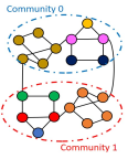
the ones locating at the top/middle/bottom of the “house” are labeled with 1,2,3, respectively. (2) BA-Community
dataset consists of two BA-Shapes graphs. Two Gaussian distributions are utilized to sample node features, one for
each BA-Shapes graph. Nodes are labeled based on their structural roles and community memberships, leading
to 8 classes in total. (3) In the Tree-Cycles dataset, an 8-level balanced binary tree is adopted as the base graph.
A set of 80 six-node cycle motifs are attached to randomly selected nodes from the base graph. (4) Tree-Grid is
constructed in the same way as TREE-CYCLES, except that 3-by-3 grid motifs are used to replace the cycle motifs. (5)
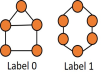
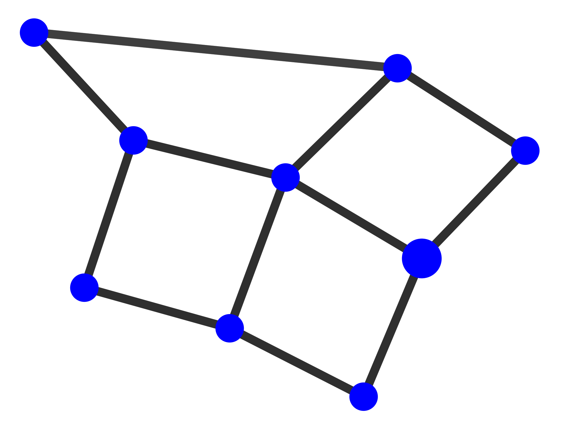
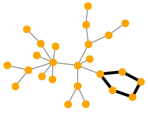
For graph classification, we build the BA-2motifs dataset of 1000 graphs. We adopt the BA graphs as base graphs.
Half graphs are attached with “house” motifs and the rest are attached with five-node cycle motifs. Graphs are
assigned to one of 2 classes according to the type of attached motifs. The first four datasets are also used in [58] for
node classification. For datasets without node features, we use a 10-dimensional vector with all elements set to
1 [58].
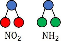
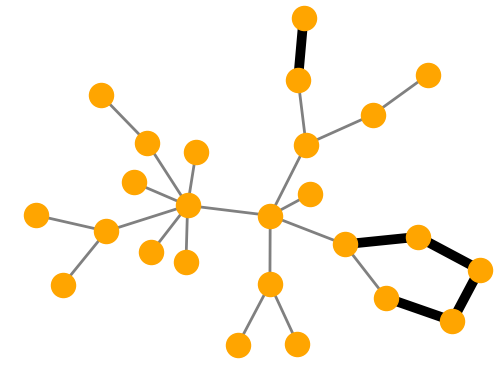
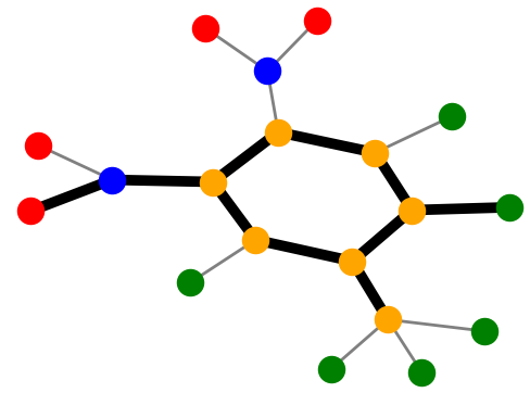
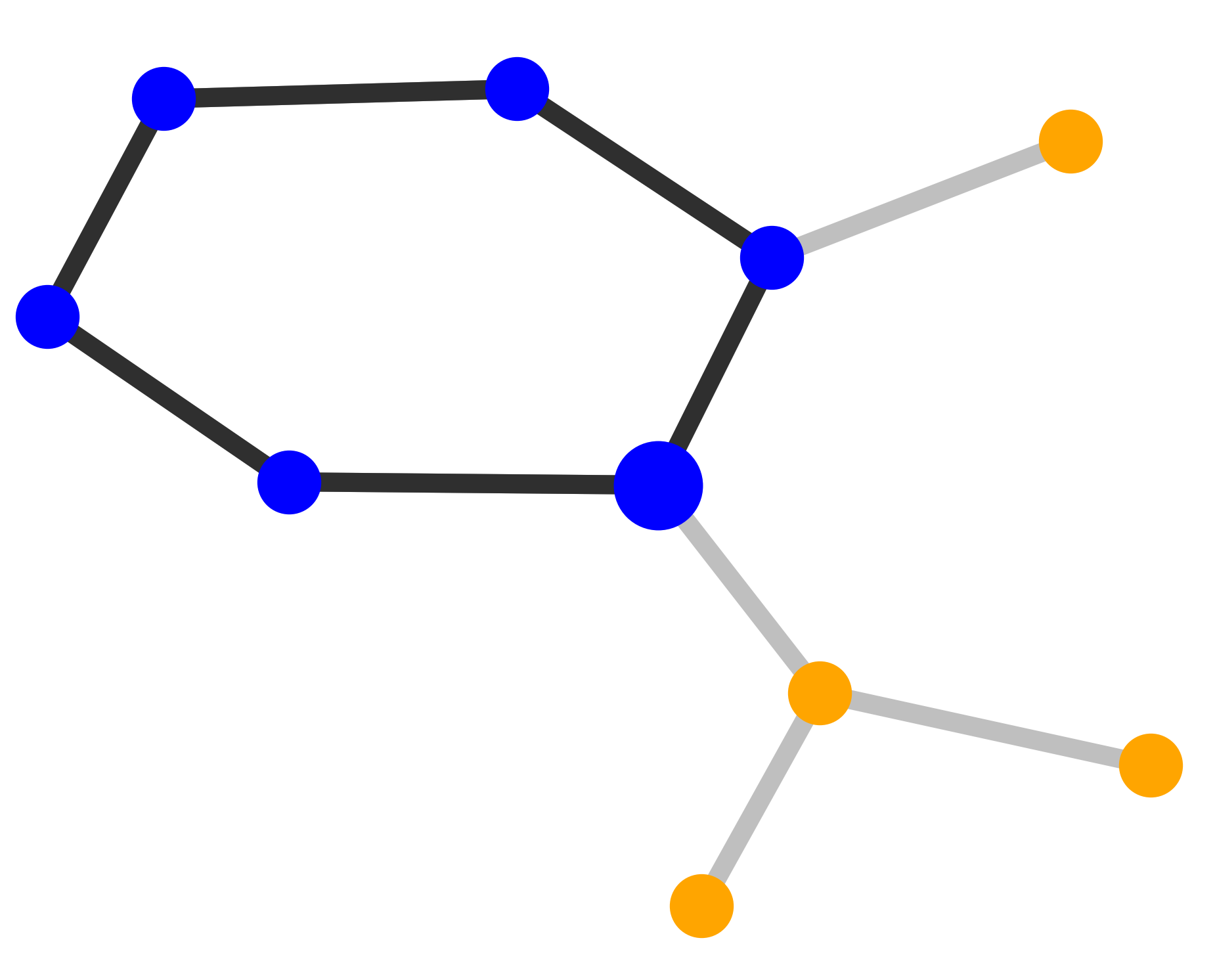
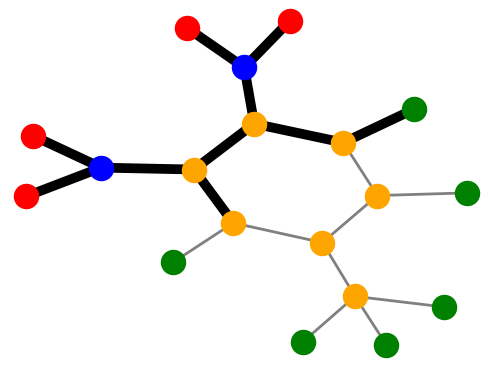
We also include a real-life dataset, MUTAG, for graph classification, which is also used in previous work [58]. It consists of 4,337
molecule graphs. Each graph is assigned to one of 2 classes based on its mutagenic effect [58, 46]. As discussed in [58, 11],
carbon rings with chemical groups NH2 or NO2 are known to be mutagenic. We observe that carbon rings exist
in both mutagen and nonmutagenic graphs, which are not discriminative. Thus, we can treat carbon rings as the
shared base graphs and NH2, NO2 as motifs for the mutagen graphs. There are no explicit motifs for nonmutagenic
ones.
Table 1 shows the statistics of synthetic and real-life datasets.
|
|
|
|
|
|
|
| | Node Classification | Graph Classification
|
| | BA-Shapes | BA-Community | Tree-Cycles | Tree-Grid | BA-2motifs | MUTAG |
|
|
|
|
|
|
|
| #graphs | 1 | 1 | 1 | 1 | 1,000 | 4,337 |
| #nodes | 700 | 1,400 | 871 | 1,231 | 25,000 | 131,488 |
| #edges | 4,110 | 8,920 | 1,950 | 3,410 | 51,392 | 266,894 |
| #labels | 4 | 8 | 2 | 2 | 2 | 2 |
|
|
|
|
|
|
|
| |
Table 1
Dataset statistics
6.2 Baselines and experimental setup
Baselines. We compare with the SOTA method, GNNExplainer as well as other baselines in [58], i.e., a gradient-based method
(GRAD), and graph attention network (ATT). (1) GNNExplainer is a post-hoc method providing explanations for every single
instance. (2) GRAD learns weights of edges by computing gradients of GNN’s objective function w.r.t. the adjacency matrix. (3) ATT
utilizes self-attention layers to distinguish edge attention weights in the input graph. Each edge’s importance is obtained by
averaging its attention weights across all attention layers.
Experimental setup. All experiments are conducted on a Linux machine with an Nvidia GeForce RTX 2070 SUPER GPU with 8GB
memory. CUDA version is 10.2 and Driver Version is 440.64.00. We follow the experimental settings in GNNExplainer [58].
Specifically, for post-hoc methods including ATT, GNNExplainer, and PGExplainer, we first train a three-layer GNN and then apply
these methods to explain predictions made by the GNN. For a fair comparison, we exactly use the specially designed GNN model in
GNNExplainer [58]. Each GNN layer is represented by f(H(l),A) = σ(W(l)AH(l)), where H(l) is the hidden representations of
nodes in the l-th layer, A is the normalized Laplacian matrix, and W(l) is the weight matrix. We adopt the Adam optimizer with
an initial learning rate of 1.0 × 10⁻³. All variables are initialized with Xavier. We follow GNNExplainer to split
train/validation/test with 80/10/10% for all datasets. Each model is trained for 1000 epochs. The accuracy performances of GNN
models are shown in Table 2. The results show that the designed GNN models are powerful enough for node/graph
classifications on both synthetic and real-life datasets. Since weights in attention layers are jointly optimized with the GNN
model in ATT, we thus train another GNN model with self-attention layers. We follow [1] to tune temperature
τ.
|
|
|
|
|
|
|
| | Node Classification | Graph Classification
|
| Accuracy | BA-Shapes | BA-Community | Tree-Cycles | Tree-Grid | BA-2motifs | MUTAG |
|
|
|
|
|
|
|
| Training | 0.98 | 0.99 | 0.99 | 0.92 | 1.00 | 0.87 |
| Validation | 1.00 | 0.88 | 1.00 | 0.94 | 1.00 | 0.89 |
| Testing | 0.97 | 0.93 | 0.99 | 0.94 | 1.00 | 0.87 |
|
|
|
|
|
|
|
| |
Table 2
Accuracy performance of GNN models
The network structure of explanation networks in PGExplainer is MLPs with one hidden layer. To train PGExplainer, we also
adopt the Adam optimizer with the initial learning rate of 3.0 × 10⁻³. The coefficient of size regularization is set to 0.05 and entropy
regularization is 1.0. The epoch T is set to 30 for all datasets. The temperature τ in Eq. (4) is set with an annealing schedule [1]:
τ(t) = τ0(τT∕τ0)t, where τ0 and τT are the initial and final temperatures. A small temperature tends to generate more discrete
graphs which may hinder the explanation network from being optimized with backpropagation. In this task, we find that relatively
high temperatures work well in practice.
| | Node Classification | Graph Classification
|
| | BA-Shapes | BA-Community | Tree-Cycles | Tree-Grid | BA-2motifs | MUTAG |
| Base | 
| | 
| 
| 
| 
|
| Motifs | 
| | 
| 
| 
| 
|
| Features | None | (μl,σl) | None | None | None | Atom types |
| Visualization |
| Explanations
by GNN-
Explainer | 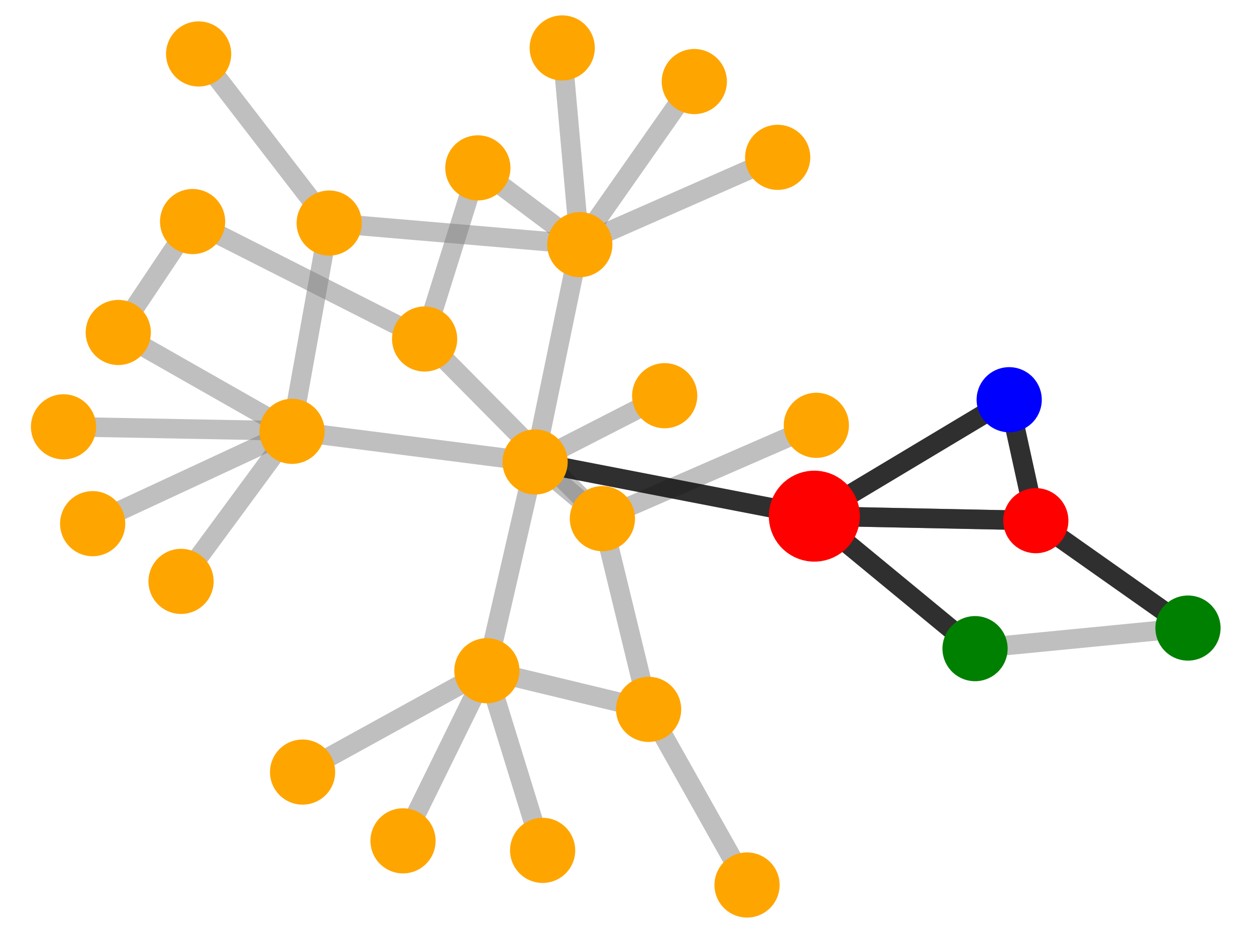
| 
| 
| 
| 
| 
|
| Explanations
by PG-
Explainer | 
| 
| 
| 
| 
| 
|
| Explanation AUC
|
|
|
|
|
|
|
|
| GRAD | 0.882 | 0.750 | 0.905 | 0.667 | 0.717 | 0.783 |
|
|
|
|
|
|
|
| ATT | 0.815 | 0.739 | 0.824 | 0.612 | 0.674 | 0.765 |
|
|
|
|
|
|
|
| Gradient | - | - | - | - | 0.773 | 0.653 |
|
|
|
|
|
|
|
| GNNExplainer | 0.925 | 0.836 | 0.948 | 0.875 | 0.742 ± 0.001 | 0.727 ± 0.014 |
|
|
|
|
|
|
|
| PGExplainer | 0.963±0.011 | 0.945±0.019 | 0.987±0.007 | 0.907±0.014 | 0.926±0.021 | 0.873±0.013 |
|
|
|
|
|
|
|
| Improve | 4.1% | 13.0% | 4.1% | 3.7% | 24.7% | 11.5% |
|
|
|
|
|
|
|
| AVG. Time (ms)
|
|
|
|
|
|
|
|
| GNNExplainer | 650.60 | 696.61 | 690.13 | 713.40 | 934.72 | 409.98 |
|
|
|
|
|
|
|
| PGExplainer
(w/
Training) | 4.62e3 | 2.54e4 | 6.09e3 | 1.85e4 | 9.87e3 | 4.26e4 |
| PGExplainer
(Inference) | 10.92 | 24.07 | 6.36 | 6.72 | 80.13 | 9.68 |
|
|
|
|
|
|
|
| Speed-up | 59x | 29x | 108x | 106x | 12x | 42x |
| |
Table 3
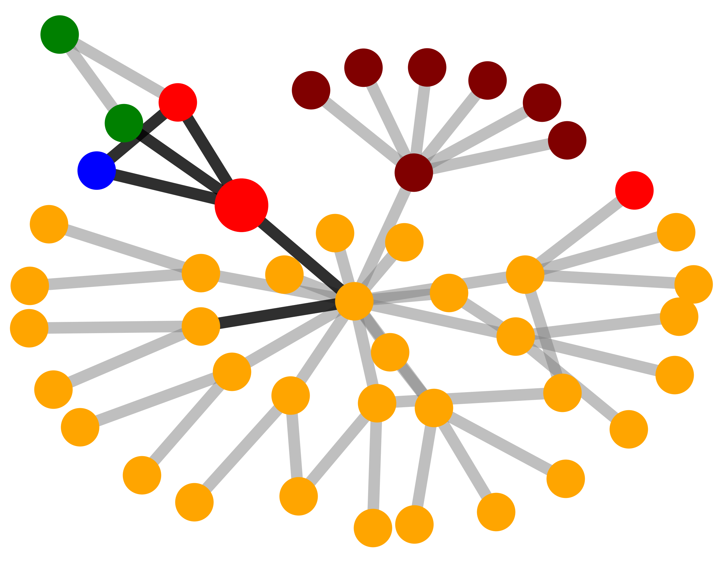
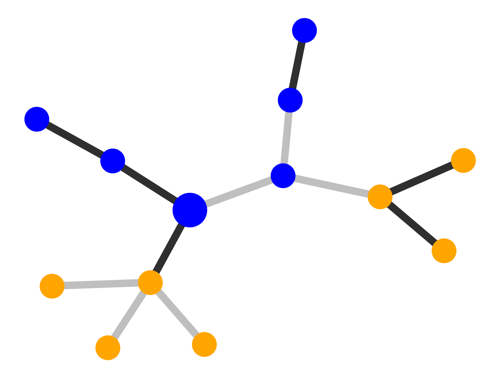
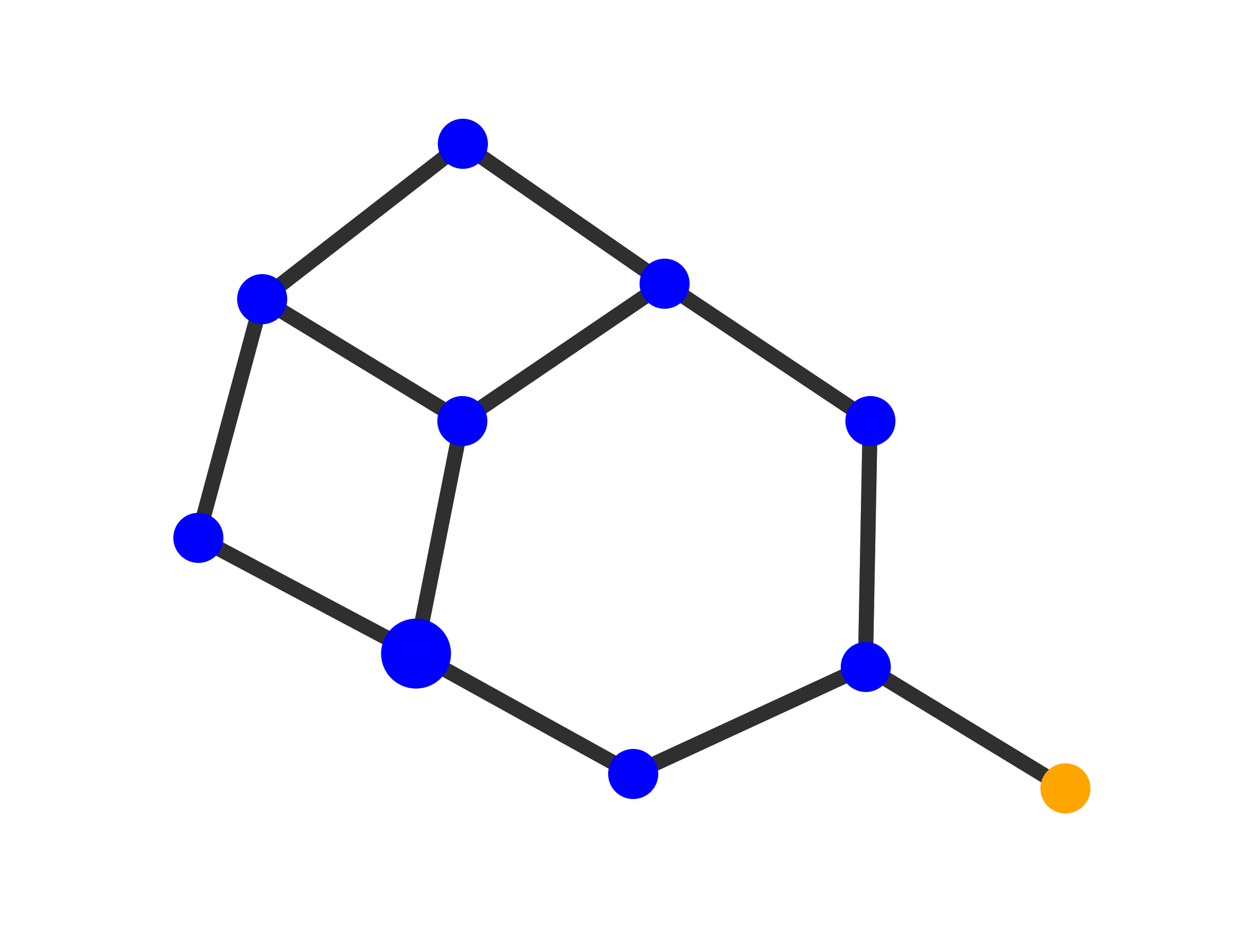
Illustration of different datasets together with performance evaluation of PGExplainer and other baselines. BA-Shapes, BA-Community,
Tree-Cycles, Tree-Grid are datasets for node classification [58]. Node labels are represented by their colors. BA-2motifs and MUTAG datasets are
used for graph classification. Graphs with “house” motifs are labeled with 0 and the ones with cycles are with 1 in BA-2motifs dataset. NH2, NO2
are treated as motifs of the mutagen graphs in MUTAG. Explanations extracted by GNNExplainer and PGExplainer are also shown as case
studies.
6.3 Comparison with Baselines
The results of comparative evaluation experiments on both synthetic and real-life datasets are summarized in Table 3. In these
datasets, node/graph labels are determined by the motifs, which are treated as ground truth explanations. These motifs are utilized
to calculate explanation accuracy for PGExplainer as well as other baselines.
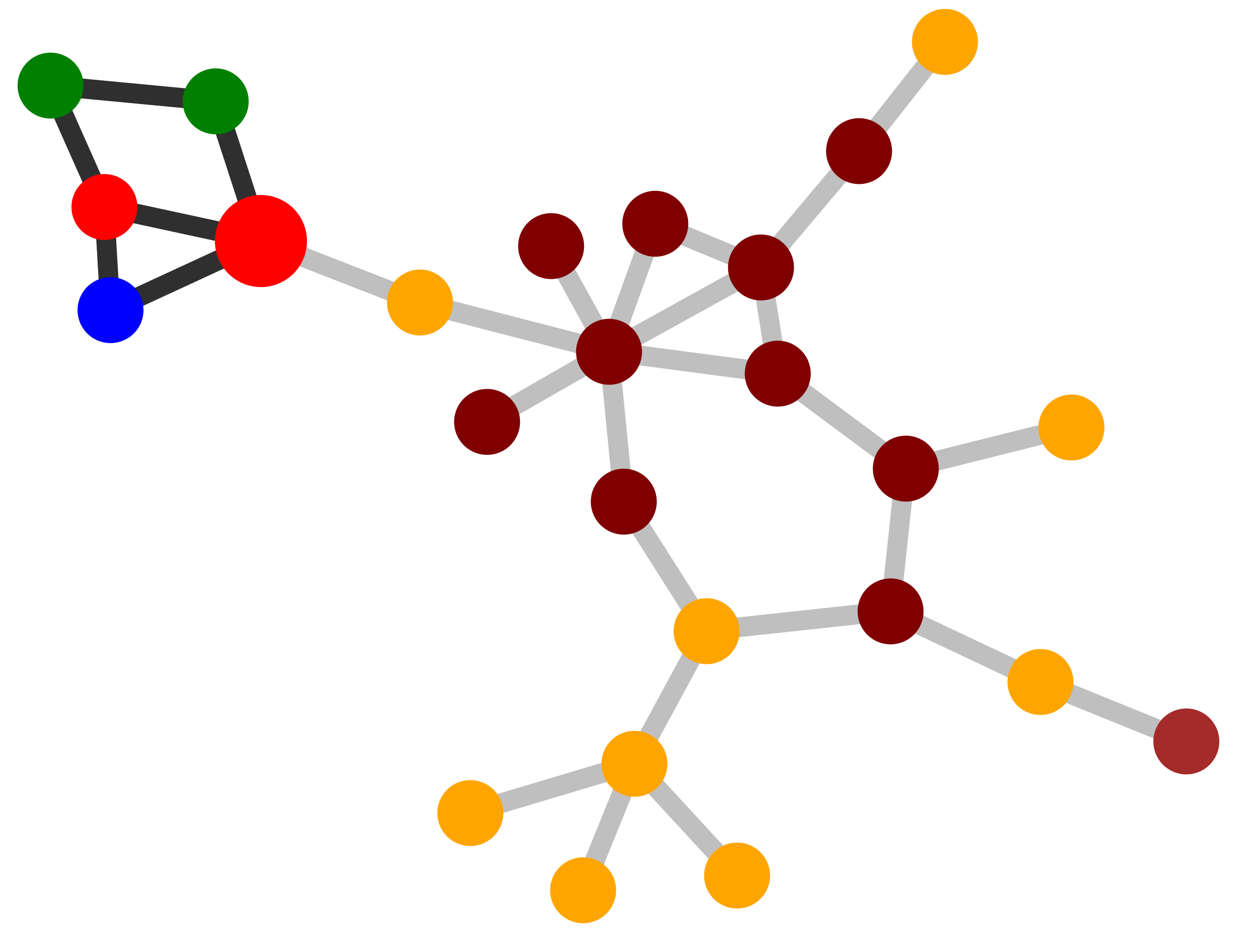
Qualitative evaluation. We choose an instance for each dataset and visualize its explanations given by GNNExplainer and
PGExplainer in Table 3. In these explanations, bold black edges indicate top-K edges ranked by their importance weights, where K
is set to the number of edges inside motifs for synthetic datasets and 10 for MUTAG [58]. As demonstrated in these figures, the
whole motifs, such as “house” in BA-Shapes and BA-Community, cycles in Tree-Cycles and BA-2motifs, grids in Tree-Grid, and
NO2 groups in MUTAG are correctly identified by PGExplainer. On the other hand, some important edges are missing in the
explanations given by GNNExplainer. For example, the explanation provided by GNNExplainer for the instance in MUTAG
contains the carbon rings and part of a NO2 group. However, the carbon rings appear frequently in both mutagen
and nonmutagenic graphs, which are not discriminative. Conversely, PGExplainer correctly identifies both NO2
groups.
Quantitative evaluation. We follow the experimental settings in GNNExplainer [58] and formalize the explanation problem as a
binary classification of edges. We treat edges inside motifs as positive edges, and negative otherwise. Importance weights provided
by explanation methods are considered as prediction scores. A good explanation method assigns high weights to edges in the
ground truth motifs than the ones outside. AUC is adopted as the metric for quantitative evaluation. Especially, for
the MUTAG dataset, we only consider the mutagen graphs because no explicit motifs exist in nonmutagenic ones.
For PGExplainer, we repeat each experiment 10 times and report the average AUC scores and standard deviations
here.
From the table, we have the following observations. PGExplainer achieves SOTA performances in all scenarios and the accuracy
gains are up to 13.0% in node classification and 24.7% in graph classification. Compared to GNNExplainer, which tackles instances
independently thus can only achieve suboptimal explanations, PGExplainer utilizes a parameterized explanation network based
upon graph generative model to collectively provide explanations for multiple instances. As a result, PGExplainer can provide a
global understanding of the GNNs. That answers why PGExplainer can outperform GNNExplainer by relatively large
margins.
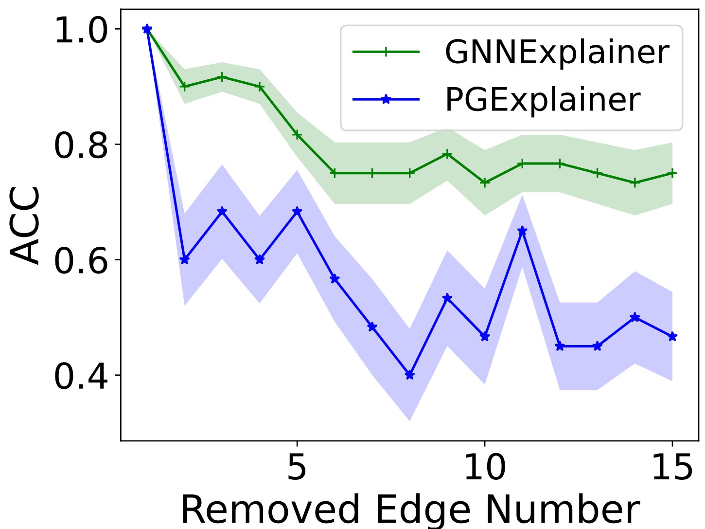
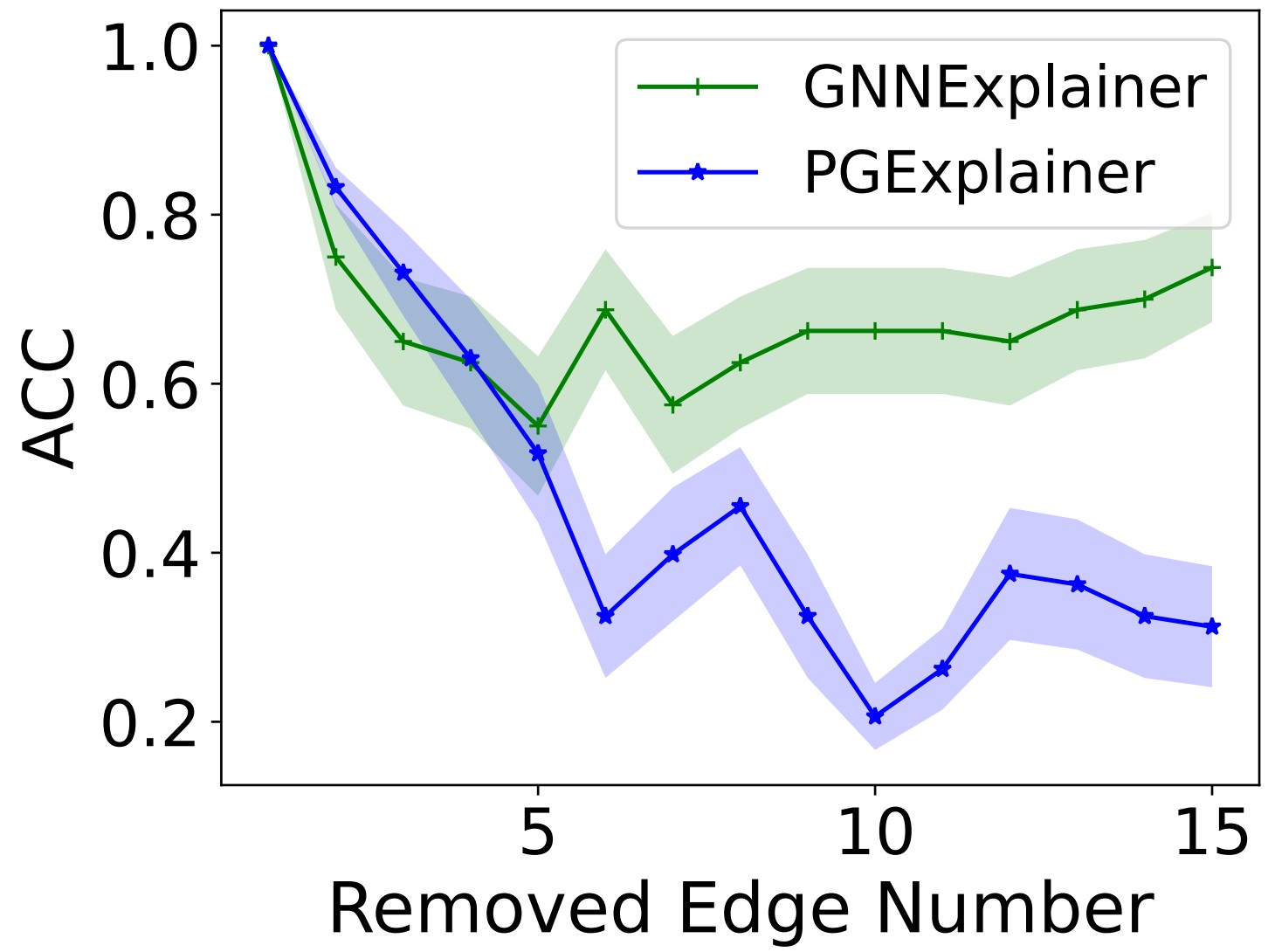
Fidelity evaluation. We adopt the experimental framework outlined in [61] for assessing the Fidelity of the generated explanations.
The Fidelity metric evaluates the degree to which the explanations genuinely reflect the model’s predictions by sequentially remove
edges based on their weights in explanation and testing the classification performance afterwards. The removal of more important
edges would degrade the classification performance more significantly. Thus, a faster performance drop would denote stronger
fidelity and better explanations.
The results on two node classification datasets, BA-Shapes and Tree-Grid, are reported in Figure 4, where we plot the curves of
model accuracy with respect to the number of removed edges. The removal of edges is ordered based on their weights in
explanation. As shown in Figure 4, PGExplainer outperforms GNNExplainer by a significant margin and show an improved
fidelity, which further verifies the effectiveness of the PGExplainer.
Efficiency evaluation. Explanation network in PGExplainer is shared across the population of instances. Thus, a trained
PGExplainer can be utilized to explain new instances in the inductive setting. We denote the time to explain a new instance with a
trained explanation method by inference time. Since GNNExplainer has to retrain the model, we also count the
training time here. The running time comparison in Table 3 shows that PGExplainer can speed up the computation
significantly, up to 108 times faster than GNNExplainer, which makes PGExplainer more practical for large-scale
datasets.
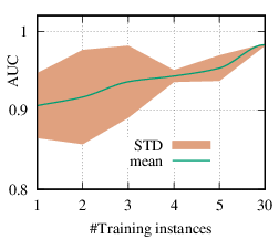
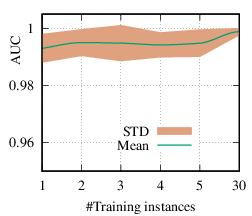
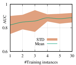
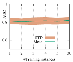
6.4 Inductive performance
As we discussed in Section 4.3, the explanation network is shared across the population. Thus, with a trained PGExplainer, we
can directly infer the explanation without retraining the explanation network. As a result, our PGExplainer has
better generalization power than the leading baseline GNNExplainer. Besides, our PGExplainer is more efficient in
the inductive setting. In this section, we empirically demonstrate the effectiveness of PGExplainer in the inductive
setting. In the inductive setting, we select α instances for training, (N - α)∕2 for validation, and the rest for testing. α
is ranged from [1,2,3,4,5,30]. Note that, with α = 1, our method degenerates to the single-instance explanation
method. Recall that to explain a set of instances, GNNExplainer first detects a reference node and then computes the
explanation for the reference node. The explanation is then generalized to other nodes with graph alignment [58]. We
claim that it may lead to sub-optimal explanations because reference node selection and graph alignment are not
jointly optimized with the explanation in an end-to-end fashion. The AUC scores of PGExplainer are shown in
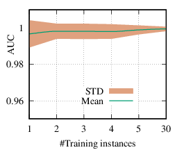
Figure 5. We have the following observations. 1) The testing AUC increase as more instances are trained, verifying the
effectiveness of PGExplainer. Some results are higher than the reported ones in Section 6 because here we adopt
validation datasets to fine-tune the hyper-parameters. 2) More training instances lead to smaller standard deviation,
PGExplainer tends to globally detect shared motifs with higher robustness. 3) PGExplainer can achieve relatively good
performance with a small number of trained instances, which makes PGExplainer more practical in large datasets.
The results also explain why we dismiss the training time of PGExplainer and only count the inference time in
Section 6.
6.5 Model Analysis.
6.5.1 Effects of regularization terms
In this part, we analyze the effects of regularization terms. In addition to the size and entropy regularizers introduced in
GNNExplainer, we also have discussed regularization terms on budgets and connectivity constraints. Since the first two
regularizers are used in the quantitative evaluation, we first conduct parameter studies. Visualization results on
synthetic datasets show that the explanatory graph extract by PGExplainer tends to be small and compact. To verify
the effectiveness of the proposed regularizer for connectivity constraint, we synthesize a noisy BA-Shapes dataset.
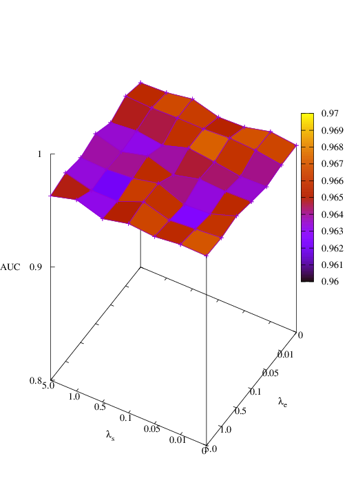
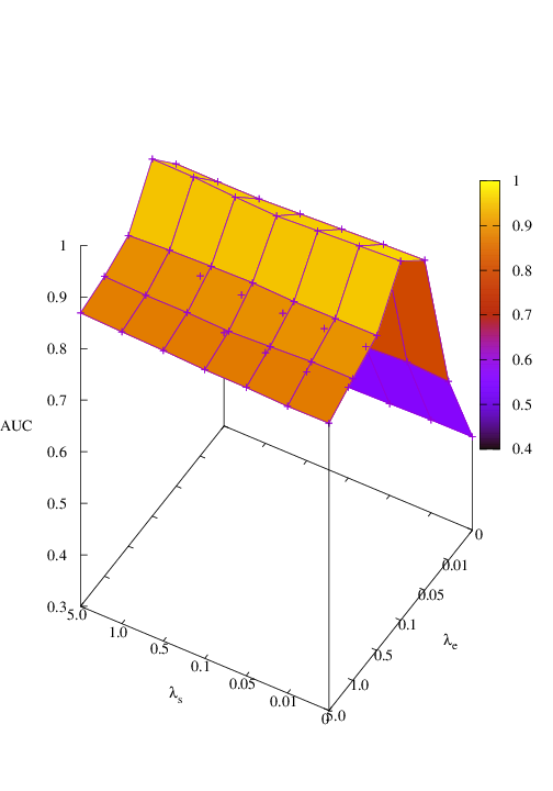
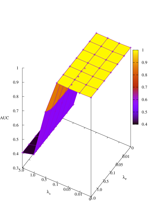
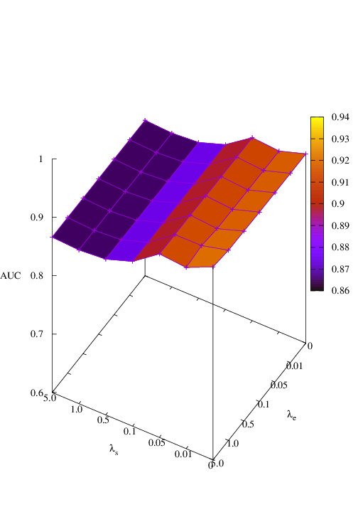
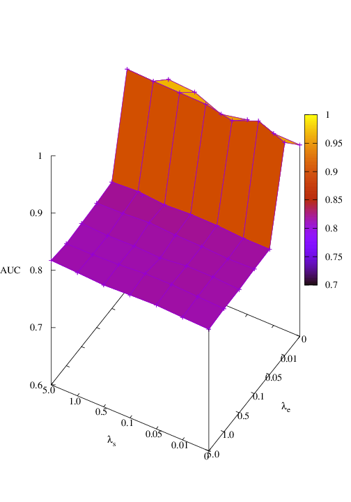
Effects of size and entropy constraint. We select synthetic datasets for parameter study. The coefficients of size and entropy
regularizers are denoted by λs and λe, respectively. AUC scores w.r.t coefficients are shown in Figure 6. We observe that
PGExplainer achieves competitive performances even without any regularization terms in all datasets except the BA-Community,
which verifies the effectiveness of the model itself. For the BA-Community dataset, the entropy constraint plays an important
role.
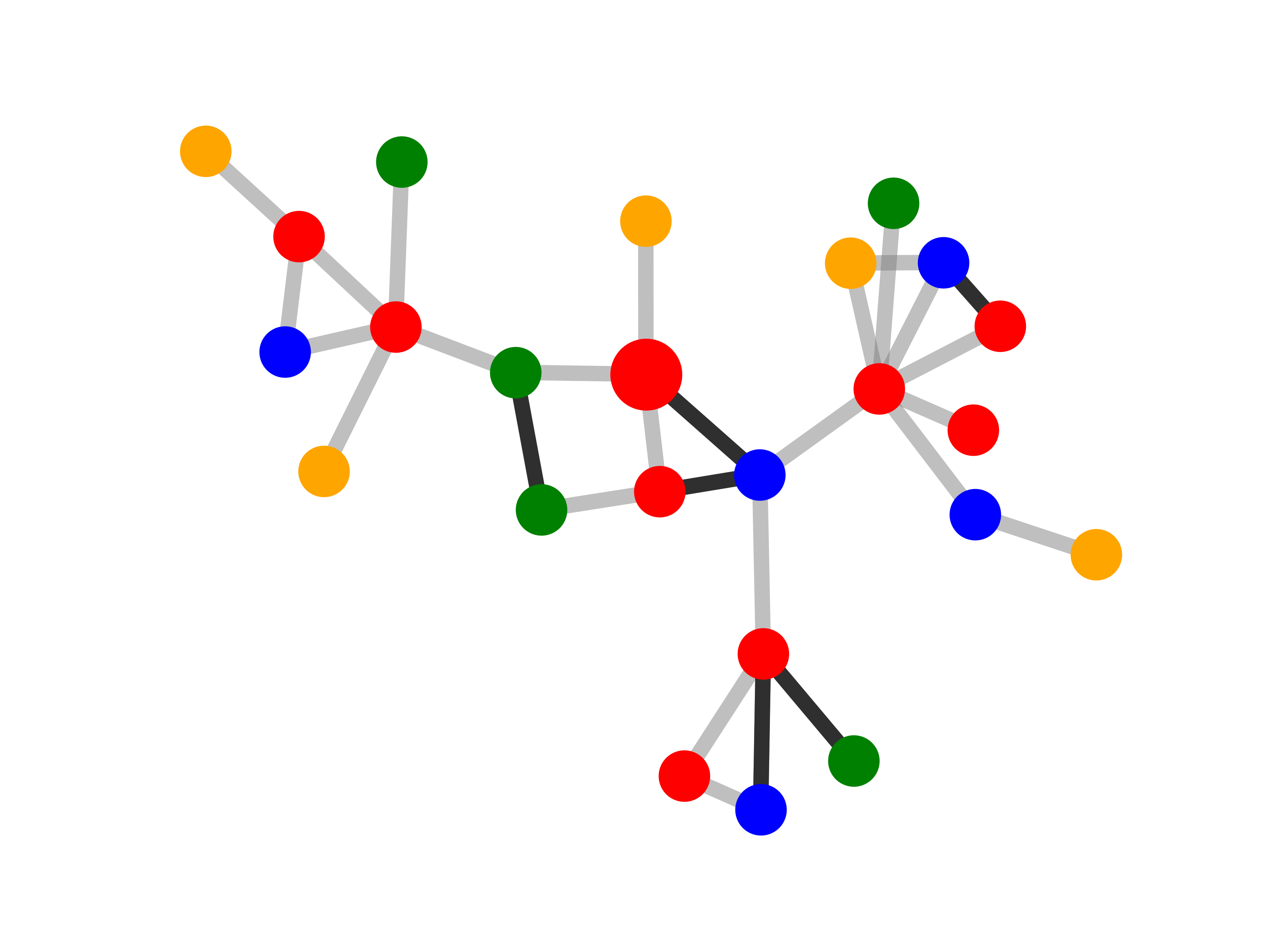
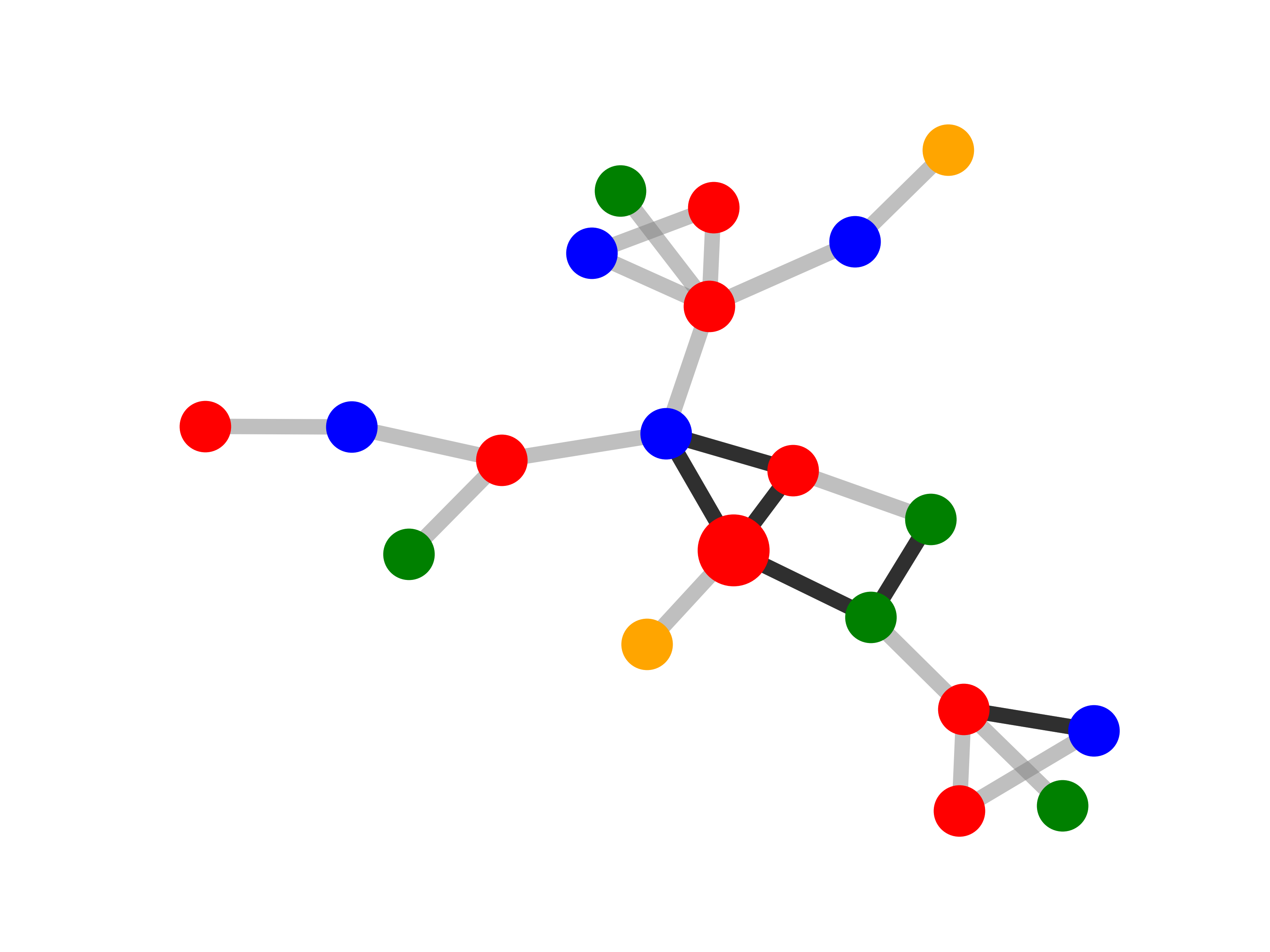
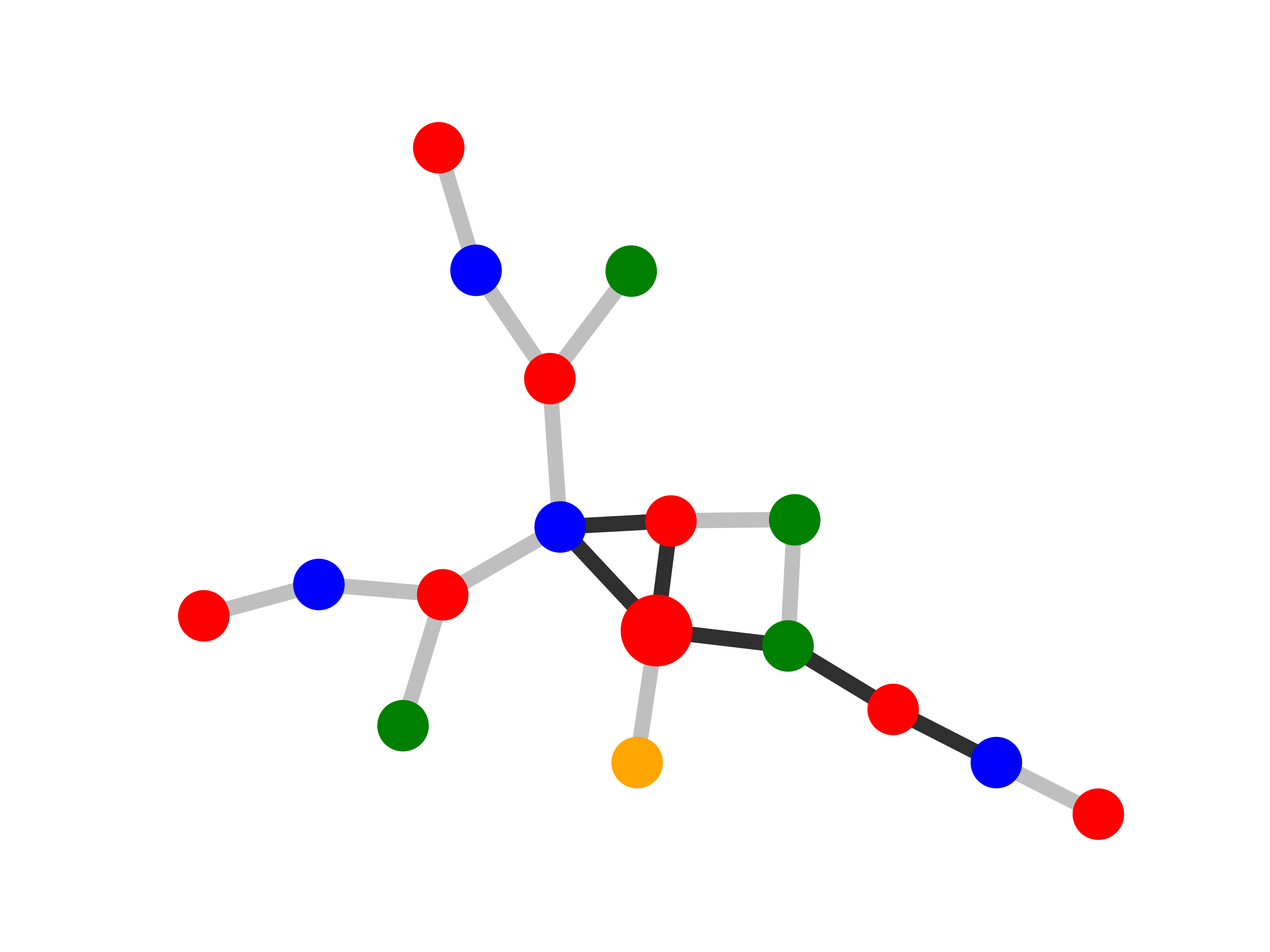
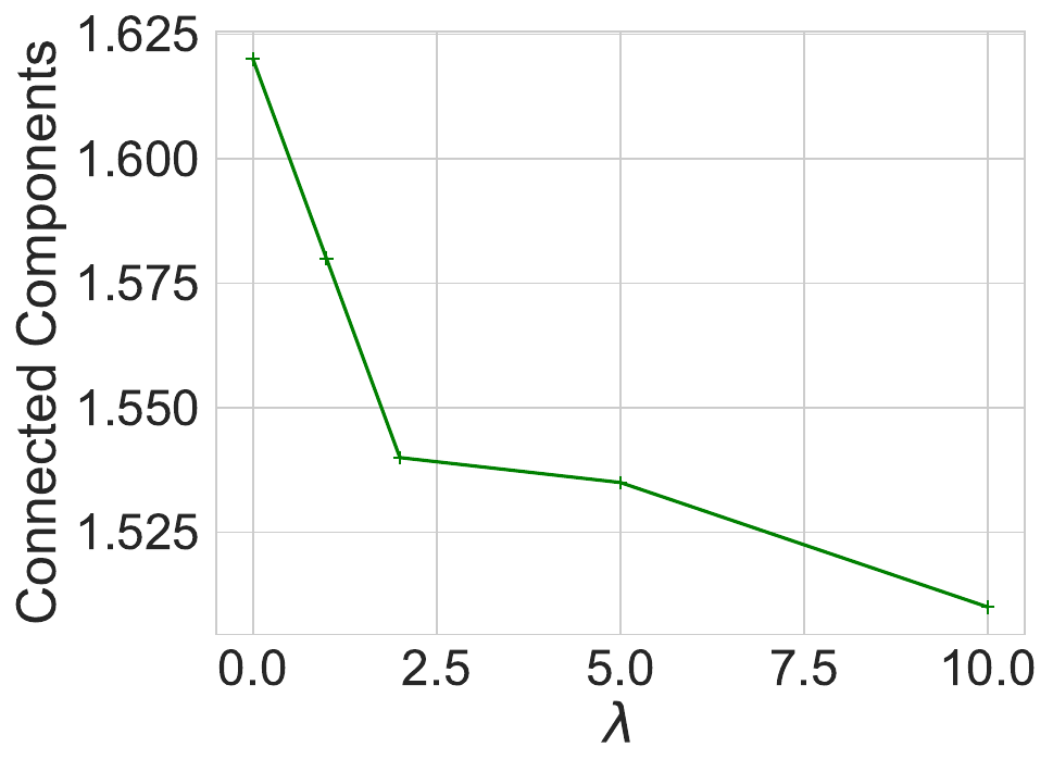
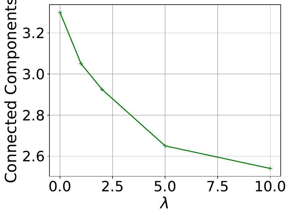
Effects of connectivity constraint. To show the effect of the connectivity constraint on the explanatory graph, we build a noisy
BA-Shapes dataset with 0.2N noisy edges and vary the coefficient of the connectivity regularization term λc from 0 to 10 and apply
PGExplainer to explain a single instance. The visualization results with regard to different choices of coefficients are shown in
Figure 7. An analysis of the number of connected components is also conducted for Tree-Cycles and Tree-Grid, with
the result presented in Figure 8. Note that in the ideal scenario, the number of connected components should be
1. Therefore, the number of connected components dropping from 1.62 to 1.50 denotes an improvement of 20%.
These figures demonstrate that without explicit constraint, PGExplainer may detect several connected edges in the
noisy input graph, although these edges are also inside motifs. With the connectivity constraint, we observe that
PGExplainer tends to reduce the number of connected components and enhance the connectivity of the explanation
subgraph.
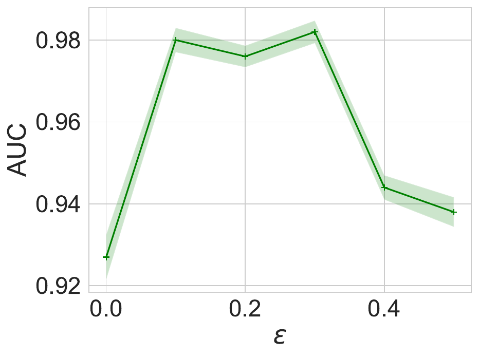
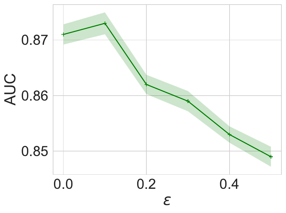
6.5.2 Effects of Stochastic Sampling.
To show the effects of the stochastic subgraph sampling, we vary the distribution range of the uniform variable ϵ in Eq. (6).
In the original PGExplainer, the independent variable ϵ is sampled from the distribution ϵ ~ Uniform(0,1). The
stochastic magnitude can be adjusted by including another hyper-parameter s, that ϵ ~ Uniform(s,1 - s), where
s ∈ [0,0.5]. A larger value of s indicates a smaller stochastic magnitude. And s = 0.5 is the deterministic version of the
PGExplainer. We adopt the Tree-Cycles and MUTAG datasets in this section and results are shown in Figure 9,
From the figure, We observe that stochastic sampling significantly and consistently improves the explanation
performances in the MUTAG datasets. With ϵ ∈ [0.1,0.3], PGExplainer outperforms its deterministic variant in the
Tree-Cycles.
6.5.3 GCN as the Backbone
To show the robustness of the PGExplainer, in this section, we compare to GNNExplainer with a representative and commonly
used GNN model, GCN [31]. Other settings are kept the same with Section 6.2. We adopt the implementations in [28]. The
accuracy performances of GCN and explanation performances of explainers are shown in Table 4.
In general, GCN works worse than the specifically designed GNN in [58]. As a result, the explanation performances of both
GNNExplainer and PGExplainer drop. However, the relative improvement of PGExplainer over GNNExplainer remains with GCN
as the backbone. PGExplainer outperforms GNNExplainer on 5 out of 6 datasets, except the Tree-Grid datasets. Specifically, AUC
gains of PGExplainer over GNNExplainer are up to 40.7% on node classification and 43.6% on graph classification, respectively,
showing the robustness of the proposed PGExplainer over the leading baseline. In addition, PGExplainer is 6 to 103 times faster than
GNNExplainer.
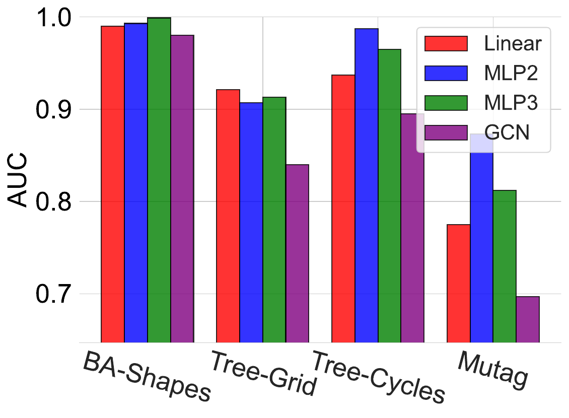
6.5.4 More Choices of Explanation Networks
In PGExplainer, we adopt a two-layer MLP as the explanation network. To show the robustness of the PGExplainer and
investigate the effects of other types of neural networks as the explainer, in this section, we include linear (Linear), MLP with
3 layers (MLP3), and GCN (GCN) to replace the vanilla MLP in PGExplainer. Results on 4 dataset are shown in
Figure 10.
From the figure, we observe that our PGExplainer is robust to the choice of explainer architectures. More sophisticated GNN
methods, such as GCN fails to further improve the explanation performances. The reason is the node embeddings used in
parameterized explainer are obtained by aggregating both node features and topological structures. Linear models and simple MLPs
are sufficient to extract informative subgraphs from them. The conclusion is aligned with the previous graph generation methods,
where simple decoders are utilized [30].
| | Node Classification | Graph Classification
|
| | BA-Shapes | BA-Community | Tree-Cycles | Tree-Grid | BA-2motifs | MUTAG |
| Accuracy performance
|
|
|
|
|
|
|
|
| Training | 0.97 | 0.75 | 0.94 | 0.91 | 0.96 | 0.82 |
| Validation | 1.00 | 0.67 | 0.98 | 0.94 | 1.00 | 0.87 |
| Testing | 1.00 | 0.71 | 0.94 | 0.93 | 0.95 | 0.80 |
|
|
|
|
|
|
|
| Explanation AUC
|
|
|
|
|
|
|
|
| GNNExplainer | 0.742±0.007 | 0.708±0.004 | 0.540±0.017 | 0.714 ± 0.003 | 0.498 ± 0.004 | 0.587 ± 0.002 |
|
|
|
|
|
|
|
| PGExplainer | 0.999±0.000 | 0.825±0.040 | 0.762±0.014 | 0.683±0.008 | 0.566±0.042 | 0.843±0.084 |
|
|
|
|
|
|
|
| Improve | 34.6% | 16.5% | 40.7% | -4.3% | 13.6% | 43.6% |
|
|
|
|
|
|
|
| Inference Time (ms)
|
|
|
|
|
|
|
|
| GNNExplainer | 412.0 | 575.5 | 360.9 | 428.3 | 218.6 | 91.7 |
|
|
|
|
|
|
|
| PGExplainer | 28.1 | 41.7 | 3.5 | 5.6 | 7.5 | 15.9 |
|
|
|
|
|
|
|
| Speed-up | 15x | 14x | 103x | 76x | 29x | 6x |
| |
Table 4
Comparison to GNNExplainer with GCN as the backbone.
|
|
|
|
|
|
| Dataset | PROTEINS | BZR_MD | Cuneiform | PTC_FR | PTC_MR |
|
|
|
|
|
|
| #graphs | 1,113 | 306 | 267 | 351 | 344 |
| Avg. # nodes | 39.06 | 21.30 | 21.27 | 14.56 | 14.29 |
| #edges | 72.82 | 225.06 | 44.80 | 15.00 | 14.69 |
| #labels | 2 | 2 | 30 | 2 | 2 |
|
|
|
|
|
|
| |
Table 5
Dataset statistics
6.6 Application to Brain Network Analysis
Analyzing the relationship between human behavioral measures and their functional brain connectivity, as measured by
resting-state functional magnetic resonance imaging (fMRI) correlations, is a fundamental task in the Neuroscience field [9, 8]. A set
of 460 subjects from the Human Connectome Project (HCP) are utilized in this case study [52], denoted by  . For each
subject s ∈, we generated the functional connectivity of brain networks using resting-state fMRI data, where nodes
denote brain regions and edges describe their functional connectivity. Each brain connectivity network is a fully
connected network with 76 nodes. Each node is associated with the cortical myelination level, which was measured by
the ratio of T1 and T2 ration [18], and cortical thickness of the corresponding region. In addition, each subject is
associated with 151 behavioral measures, including Pittsburgh Sleep Quality Index (PSQI) score, NIH Toolbox Sadness
Survey: Unadjusted Scale Score, et. al. A canonical-correlation analysis (CCA) score has been calculated for each
subject to summarize his/her position along a direction that maximally linked these behavioral measures to the
neuroimaging data [24]. Based on their CCA scores, we split the 460 subjects into two groups, “pos” and “neg”. A subject is
assigned to the “pos” set, denoted by pos if the CCA score is positive. Otherwise, s/he is assigned to the “neg” set
neg.
. For each
subject s ∈, we generated the functional connectivity of brain networks using resting-state fMRI data, where nodes
denote brain regions and edges describe their functional connectivity. Each brain connectivity network is a fully
connected network with 76 nodes. Each node is associated with the cortical myelination level, which was measured by
the ratio of T1 and T2 ration [18], and cortical thickness of the corresponding region. In addition, each subject is
associated with 151 behavioral measures, including Pittsburgh Sleep Quality Index (PSQI) score, NIH Toolbox Sadness
Survey: Unadjusted Scale Score, et. al. A canonical-correlation analysis (CCA) score has been calculated for each
subject to summarize his/her position along a direction that maximally linked these behavioral measures to the
neuroimaging data [24]. Based on their CCA scores, we split the 460 subjects into two groups, “pos” and “neg”. A subject is
assigned to the “pos” set, denoted by pos if the CCA score is positive. Otherwise, s/he is assigned to the “neg” set
neg.
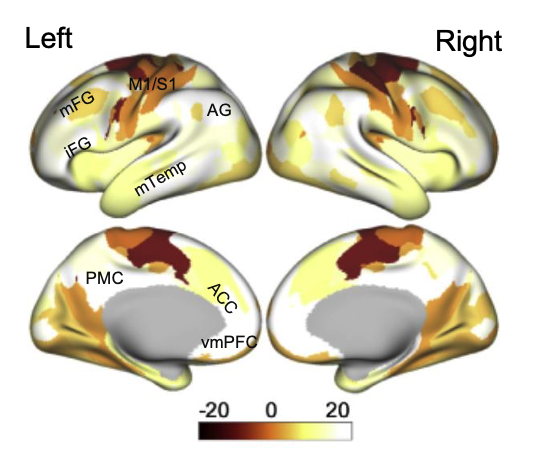
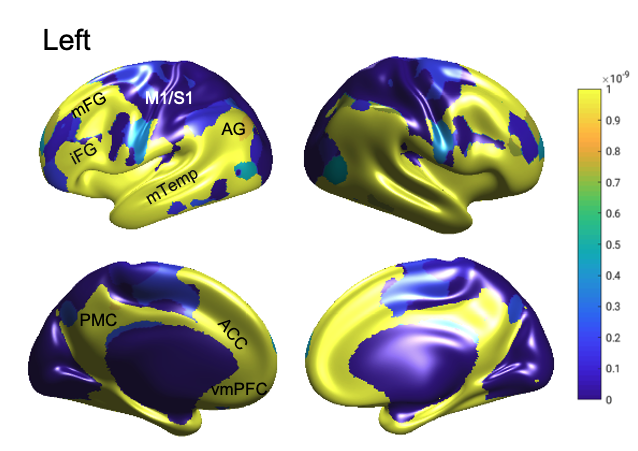
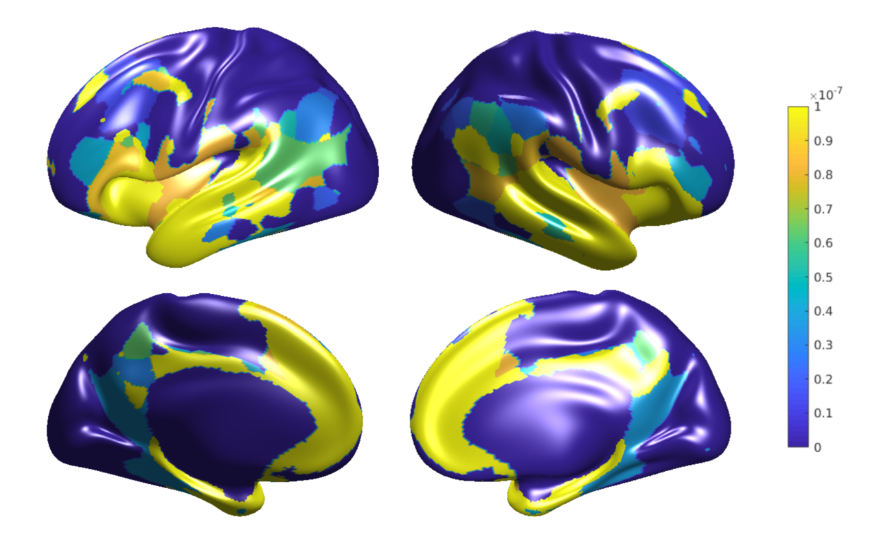
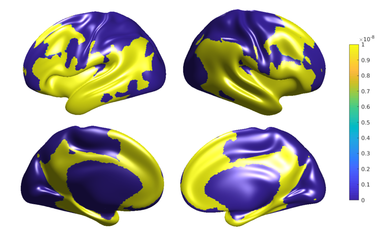
A three-layer GNN model is utilized to predict a subject’s group label based on its brain network. For subject i, we adopt
PGExplainer to learn a weight matrix Ωi ∈ℝ76×76, which measures the strength of the relationship between functional connectivity
and the subject’s behavior measurements. Specifically, the diagonal elements in Ωi reflect the importance of each brain region. To
analyze the relationship between human behaviors and brain network connectivity at a group level, we consider three groups.
Ωpos =  ∑
i∈
∑
i∈ posΩi is the average weight matrices of subjects in the “pos” set pos; Ωneg =
  ∑
i∈negΩi is for the “neg”
set; Ωall =
∑
i∈negΩi is for the “neg”
set; Ωall =  ∑
i∈Ωi is for all these 460 subjects. For each group, we extracted the diagonal elements from the corresponding
matrix and displayed the results on a brain surface. The results for these three groups are shown in Figure 11(b), 11(c), and 11(d),
respectively. Regions with yellow color are associated with higher weights, indicating critical impacts on the behavior
measurements.
∑
i∈Ωi is for all these 460 subjects. For each group, we extracted the diagonal elements from the corresponding
matrix and displayed the results on a brain surface. The results for these three groups are shown in Figure 11(b), 11(c), and 11(d),
respectively. Regions with yellow color are associated with higher weights, indicating critical impacts on the behavior
measurements.
Based on these figures, we have the following observations. First, the overall spatial patterns of the “pos”, “neg”, and “all”
groups are consistent with the patterns found by traditional canonical-correlation analysis (Figure 11(a)), especially the contrast
between the higher-order/hierarchy association regions (middle frontal gyrus [mFG], inferior frontal gyrus [iFG], angular gyrus
[AG], middle temporal cortex [mTemp], anterior cingulate cortex [ACC], posteromedial cortex [PMC], ventromedial
prefrontal cotex [vmPFC]) and lower-order primary sensory-motor networks (primary motor cortex [M1], primary
somatosensory cortex [S1]), are close to each other. Of note, this cross-hierarchy pattern was the core feature emphasized
in [24]. On the other hand, we also observe the difference between spatial patterns of “pos” and “neg” groups. To
measure the consistency quantitatively, we further calculate the Spearman’s rank correlation coefficient between the
patterns discovered by us and those by traditional analysis. Across 76 cortical regions (Figure 11(a)), we get the
correlation coefficient as 0.3346 and the p-value as 0.0031, which validate the significance of consistency between two
panels.
6.7 Self-Explainable Graph Learning
In this section, we evaluate the effectiveness of the self-explainable graph learning framework. First, we compare the
explanations achieved by the self-explainable method with post-hoc counterparts. We include GNNExplainer and PGExplainer as
baselines and report the results w.r.t both the explanation quality (in terms of AUC on edges) and classification performance (in
terms of ACCuracy), with the result in Table 6. It can be observed that our self-explainable framework can achieve
comparable or better explanation quality with PGExplainer and bring improvements to downstream classification in most
cases.
|
|
|
|
|
| | | BA-Shapes | Tree-Cycles | Tree-Grid |
|
|
|
|
|
|
AUC | GNNExpl | 0.74 | 0.54 | 0.71 |
| | PGExpl | 0.99 | 0.76 | 0.68 |
| | SelfExpl | 0.99 | 0.78 | 0.82 |
|
|
|
|
|
|
ACC | Backbone | 1.00 | 0.94 | 0.93 |
| | SelfExpl | 1.00 | 0.98 | 0.92 |
|
|
|
|
|
| |
Table 6
Performance analysis of our self-explainable learning framework.
Second, we verify the accuracy performance of the self-explain GNN method with 5 datasets from different
fields ,
including PROTEINS [3], BZR_MD [51], Cuneiform [32], PTC_FR [25] and PTC_MR [25]. Dataset statistics are shown in
Table 5.
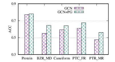
Three-layer GCNs are adopted as the backbone. Readout operation is then applied to get the graph embeddings from node
embeddings. We apply explanation networks with size constraints to the GCN, denoted by GCN+PG, and compare it to the basic
one. The comparison results are shown in Figure 12. Our GCN+PG consistently outperforms GCN in all these five datasets with up
to 17.80% achievement in classification accuracy, verifying the effectiveness of our method in the performance of graph
classification.
7 Conclusion
We present PGExplainer, a parameterized method to provide a global understanding of any GNN models on arbitrary machine
learning tasks by collectively explaining multiple instances. We show that PGExplainer can leverage the representations produced
by GNNs to learn the underlying subgraphs that are important to the predictions made by them. Furthermore, PGExplainer is more
efficient due to its capacity to explain GNNs in inductive settings, which makes PGExplainer more practical in real-life applications.
In addition, we show that the explanation network with size constraint can also extract informative structures in the input graph to
improve the performance of GNNs.
Acknowledgement
This project was partially supported by NSF projects IIS-1707548 and CBET-1638320.
References
[1] Abubakar Abid, Muhammad Fatih Balin, and James Zou. Concrete autoencoders for differentiable feature selection and reconstruction.
arXiv preprint arXiv:1901.09346, 2019.
[2] Raman Arora and Jalaj Upadhyay. On differentially private graph sparsification and applications. In NeurIPS, pages 13378–13389, 2019.
[3] Karsten M Borgwardt, Cheng Soon Ong, Stefan Schönauer, SVN Vishwanathan, Alex J Smola, and Hans-Peter Kriegel. Protein function
prediction via graph kernels. Bioinformatics, 21(suppl_1):i47–i56, 2005.
[4] Joan Bruna, Wojciech Zaremba, Arthur Szlam, and Yann LeCun. Spectral networks and locally connected networks on graphs. arXiv
preprint arXiv:1312.6203, 2013.
[5] Rich Caruana, Yin Lou, Johannes Gehrke, Paul Koch, Marc Sturm, and Noemie Elhadad. Intelligible models for healthcare: Predicting
pneumonia risk and hospital 30-day readmission. In KDD, pages 1721–1730, 2015.
[6] Jianbo Chen, Le Song, Martin Wainwright, and Michael Jordan. Learning to explain: An information-theoretic perspective on model
interpretation. In ICML, pages 883–892. PMLR, 2018.
[7] L Paul Chew. There are planar graphs almost as good as the complete graph. Journal of Computer and System Sciences, 39(2):205–219, 1989.
[8] Hejie Cui, Wei Dai, Yanqiao Zhu, Xuan Kan, Antonio Aodong Chen Gu, Joshua Lukemire, Liang Zhan, Lifang He, Ying Guo, and Carl
Yang. Braingb: a benchmark for brain network analysis with graph neural networks. IEEE Transactions on Medical Imaging, 2022.
[9] Hejie Cui, Wei Dai, Yanqiao Zhu, Xiaoxiao Li, Lifang He, and Carl Yang. Interpretable graph neural networks for connectome-based
brain disorder analysis. In Medical Image Computing and Computer Assisted Intervention–MICCAI 2022: 25th International Conference, Singapore,
September 18–22, 2022, Proceedings, Part VIII, pages 375–385. Springer, 2022.
[10] Piotr Dabkowski and Yarin Gal. Real time image saliency for black box classifiers. In NIPS, pages 6967–6976, 2017.
[11] Asim Kumar Debnath, Rosa L Lopez de Compadre, Gargi Debnath, Alan J Shusterman, and Corwin Hansch. Structure-activity
relationship of mutagenic aromatic and heteroaromatic nitro compounds. correlation with molecular orbital energies and hydrophobicity.
Journal of medicinal chemistry, 34(2):786–797, 1991.
[12] Michaël Defferrard, Xavier Bresson, and Pierre Vandergheynst. Convolutional neural networks on graphs with fast localized spectral
filtering. In NIPS, pages 3844–3852, 2016.
[13] P ERDdS and A R&wi. On random graphs i. Publ. Math. Debrecen, 6(290-297):18, 1959.
[14] D. Erhan, Y. Bengio, A. Courville, and P. Vincent. Visualizing higher-layer features of a deep network. University of Montreal, 1341(3):1,
2019.
[15] Ruth C Fong and Andrea Vedaldi. Interpretable explanations of black boxes by meaningful perturbation. In ICCV, pages 3429–3437,
2017.
[16] Edgar N Gilbert. Random graphs. The Annals of Mathematical Statistics, 30(4):1141–1144, 1959.
[17] Justin Gilmer, Samuel S Schoenholz, Patrick F Riley, Oriol Vinyals, and George E Dahl. Neural message passing for quantum chemistry.
In ICML, pages 1263–1272, 2017.
[18] Matthew F Glasser and David C Van Essen. Mapping human cortical areas in vivo based on myelin content as revealed by t1-and
t2-weighted mri. Journal of Neuroscience, 31(32):11597–11616, 2011.
[19] Marco Gori, Gabriele Monfardini, and Franco Scarselli. A new model for learning in graph domains. In IJCNN, volume 2, pages 729–734.
IEEE, 2005.
[20] Aditya Grover, Aaron Zweig, and Stefano Ermon. Graphite: Iterative generative modeling of graphs. In ICML, 2019.
[21] Wenbo Guo, Sui Huang, Yunzhe Tao, Xinyu Xing, and Lin Lin. Explaining deep learning models–a bayesian non-parametric approach.
In NeurIPS, pages 4514–4524, 2018.
[22] Wenbo Guo, Dongliang Mu, Jun Xu, Purui Su, Gang Wang, and Xinyu Xing. Lemna: Explaining deep learning based security applications.
In CCS, pages 364–379, 2018.
[23] Will Hamilton, Zhitao Ying, and Jure Leskovec. Inductive representation learning on large graphs. In NIPS, pages 1024–1034, 2017.
[24] Feng Han, Yameng Gu, Gregory L Brown, Xiang Zhang, and Xiao Liu. Neuroimaging contrast across the cortical hierarchy is the feature
maximally linked to behavior and demographics. Neuroimage, 215:116853, 2020.
[25] Christoph Helma, Ross D. King, Stefan Kramer, and Ashwin Srinivasan. The predictive toxicology challenge 2000–2001. Bioinformatics,
17(1):107–108, 2001.
[26] Gecia Bravo Hermsdorff and Lee M Gunderson. A unifying framework for spectrum-preserving graph sparsification and coarsening.
arXiv preprint arXiv:1902.09702, 2019.
[27] Peter D Hoff, Adrian E Raftery, and Mark S Handcock. Latent space approaches to social network analysis. Journal of the american
Statistical association, 97(460):1090–1098, 2002.
[28] Lars Holdijk, Maarten Boon, Stijn Henckens, and Lysander de Jong. [re] parameterized explainer for graph neural network. In ML
Reproducibility Challenge 2020, 2021.
[29] Eric Jang, Shixiang Gu, and Ben Poole. Categorical reparameterization with gumbel-softmax. ICLR, 2017.
[30] Thomas N Kipf and Max Welling. Variational graph auto-encoders. arXiv preprint arXiv:1611.07308, 2016.
[31] Thomas N Kipf and Max Welling. Semi-supervised classification with graph convolutional networks. ICLR, 2017.
[32] Nils M Kriege, Matthias Fey, Denis Fisseler, Petra Mutzel, and Frank Weichert. Recognizing cuneiform signs using graph based methods.
In International Workshop on Cost-Sensitive Learning, pages 31–44. PMLR, 2018.
[33] Himabindu Lakkaraju, Ece Kamar, Rich Caruana, and Jure Leskovec. Interpretable & explorable approximations of black box models.
CoRR, abs/1707.01154, 2017.
[34] Jure Leskovec, Jon Kleinberg, and Christos Faloutsos. Graphs over time: densification laws, shrinking diameters and possible
explanations. In KDD, pages 177–187, 2005.
[35] Jiwei Li, Will Monroe, and Dan Jurafsky. Understanding neural networks through representation erasure. arXiv preprint arXiv:1612.08220,
2016.
[36] Ruoyu Li, Sheng Wang, Feiyun Zhu, and Junzhou Huang. Adaptive graph convolutional neural networks. In AAAI, 2018.
[37] Scott Lundberg and Su-In Lee. A unified approach to interpreting model predictions. NIPS, 2017.
[38] Scott M Lundberg and Su-In Lee. A unified approach to interpreting model predictions. In NIPS, pages 4765–4774, 2017.
[39] Dongsheng Luo, Wei Cheng, Wenchao Yu, Bo Zong, Jingchao Ni, Haifeng Chen, and Xiang Zhang. Learning to drop: Robust graph
neural network via topological denoising. In WSDM, pages 779–787, 2021.
[40] Jianxin Ma, Peng Cui, Kun Kuang, Xin Wang, and Wenwu Zhu. Disentangled graph convolutional networks. In ICML, pages 4212–4221,
2019.
[41] Jiaqi Ma, Weijing Tang, Ji Zhu, and Qiaozhu Mei. A flexible generative framework for graph-based semi-supervised learning. In NeurIPS,
pages 3276–3285, 2019.
[42] Chris J Maddison, Andriy Mnih, and Yee Whye Teh. The concrete distribution: A continuous relaxation of discrete random variables.
ICLR, 2017.
[43] Mark Newman. Networks. Oxford university press, 2018.
[44] Jingchao Ni, Shiyu Chang, Xiao Liu, Wei Cheng, Haifeng Chen, Dongkuan Xu, and Xiang Zhang. Co-regularized deep multi-network
embedding. In WWW, 2018.
[45] Marco Tulio Ribeiro, Sameer Singh, and Carlos Guestrin. ” why should i trust you?” explaining the predictions of any classifier. In KDD,
pages 1135–1144, 2016.
[46] Kaspar Riesen and Horst Bunke. Iam graph database repository for graph based pattern recognition and machine learning. In Joint
IAPR International Workshops on Statistical Techniques in Pattern Recognition (SPR) and Structural and Syntactic Pattern Recognition (SSPR), pages
287–297. Springer, 2008.
[47] Franco Scarselli, Marco Gori, Ah Chung Tsoi, Markus Hagenbuchner, and Gabriele Monfardini. The graph neural network model. IEEE
TNN, 20(1):61–80, 2008.
[48] Avanti Shrikumar, Peyton Greenside, and Anshul Kundaje. Learning important features through propagating activation differences. In
ICML, pages 3145–3153. PMLR, 2017.
[49] David I Shuman, Sunil K Narang, Pascal Frossard, Antonio Ortega, and Pierre Vandergheynst. The emerging field of signal processing
on graphs: Extending high-dimensional data analysis to networks and other irregular domains. IEEE signal processing magazine, 30(3):83–98,
2013.
[50] Mukund Sundararajan, Ankur Taly, and Qiqi Yan. Axiomatic attribution for deep networks. ICML, 2017.
[51] Jeffrey J Sutherland, Lee A O’brien, and Donald F Weaver. Spline-fitting with a genetic algorithm: A method for developing classification
structure- activity relationships. Journal of chemical information and computer sciences, 43(6):1906–1915, 2003.
[52] David C Van Essen, Stephen M Smith, Deanna M Barch, Timothy EJ Behrens, Essa Yacoub, Kamil Ugurbil, Wu-Minn HCP Consortium,
et al. The wu-minn human connectome project: an overview. Neuroimage, 2013.
[53] Petar Veličković, Guillem Cucurull, Arantxa Casanova, Adriana Romero, Pietro Lio, and Yoshua Bengio. Graph attention networks. ICLR,
2018.
[54] Chi-Jen Wang, Seokjoo Chae, Leonid A Bunimovich, and Benjamin Z Webb. Uncovering hierarchical structure in social networks using
isospectral reductions. arXiv preprint arXiv:1801.03385, 2017.
[55] Keyulu Xu, Weihua Hu, Jure Leskovec, and Stefanie Jegelka. How powerful are graph neural networks? ICLR, 2019.
[56] Chengliang Yang, Anand Rangarajan, and Sanjay Ranka. Global model interpretation via recursive partitioning. In HPCC, pages
1563–1570. IEEE, 2018.
[57] Rex Ying, Ruining He, Kaifeng Chen, Pong Eksombatchai, William L Hamilton, and Jure Leskovec. Graph convolutional neural networks
for web-scale recommender systems. In KDD, pages 974–983, 2018.
[58] Zhitao Ying, Dylan Bourgeois, Jiaxuan You, Marinka Zitnik, and Jure Leskovec. Gnnexplainer: Generating explanations for graph neural
networks. In NeurIPS, pages 9240–9251, 2019.
[59] Jiaxuan You, Rex Ying, Xiang Ren, William L Hamilton, and Jure Leskovec. Graphrnn: Generating realistic graphs with deep
auto-regressive models. In ICML, 2018.
[60] Hao Yuan, Jiliang Tang, Xia Hu, and Shuiwang Ji. Xgnn: Towards model-level explanations of graph neural networks. In SIGKDD, pages
430–438, 2020.
[61] Hao Yuan, Haiyang Yu, Shurui Gui, and Shuiwang Ji. Explainability in graph neural networks: A taxonomic survey. arXiv preprint
arXiv:2012.15445, 2020.
[62] Hao Yuan, Haiyang Yu, Jie Wang, Kang Li, and Shuiwang Ji. On explainability of graph neural networks via subgraph explorations.
arXiv preprint arXiv:2102.05152, 2021.
[63] Muhan Zhang and Yixin Chen. Link prediction based on graph neural networks. In NIPS, pages 5165–5175, 2018.
[64] Tianxiang Zhao, Dongsheng Luo, Xiang Zhang, and Suhang Wang. Faithful and consistent graph neural network explanations with
rationale alignment. arXiv preprint arXiv:2301.02791, 2023.
[65] Tianxiang Zhao, Dongsheng Luo, Xiang Zhang, and Suhang Wang. Towards faithful and consistent explanations for graph neural
networks. In Proceedings of the Sixteenth ACM International Conference on Web Search and Data Mining, pages 634–642, 2023.
[66] Cheng Zheng, Bo Zong, Wei Cheng, Dongjin Song, Jingchao Ni, Wenchao Yu, Haifeng Chen, and Wei Wang. Robust graph representation
learning via neural sparsification. In ICML, pages 11458–11468. PMLR, 2020.
[67] Yanqiao Zhu, Weizhi Xu, Jinghao Zhang, Qiang Liu, Shu Wu, and Liang Wang. Deep graph structure learning for robust representations:
A survey. arXiv preprint arXiv:2103.03036, 2021.
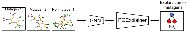

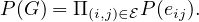
![mGisnH (Yo|G = Gs ) = miGns EGs[H (Yo|G = Gs )]
≈ min EGs~q(Θ )[H (Yo|G = Gs)]
Θ](Main2x.png)

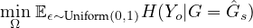
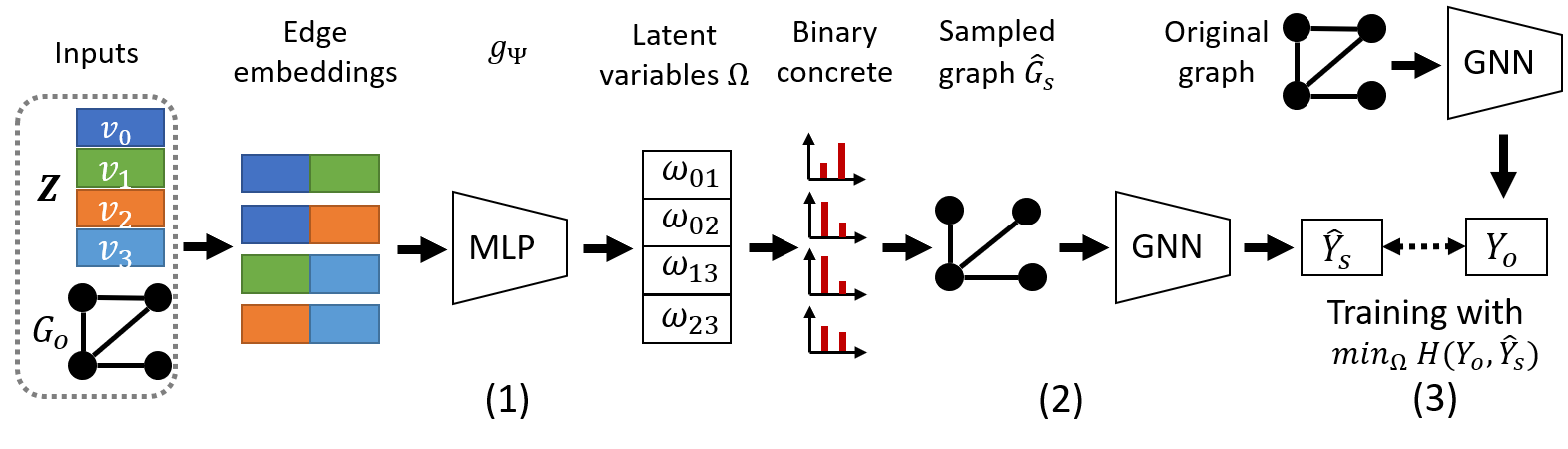

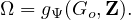
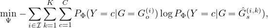
![ωij = M LPΨ([zi;zj;zv]).](Main12x.png)
![ωij = M LPΨ ([zi;zj]).](Main13x.png)
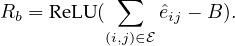
![H (ˆeij,ˆeik) = - [(1 - θij)log(1 - θik)+ θijlogθik],](Main15x.png)

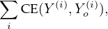
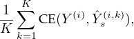
![K
∑ [CE(Y(i),Y (i))+ 1-∑ (CE(Y(i), ˆY(i,k))].
i o K k=1 s](Main19x.png)