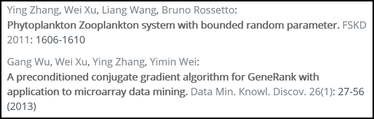
Figure 1. Example taken from DBLP
A Collective Approach to Scholar Name Disambiguation
Dongsheng Luo, Shuai Ma, Yaowei Yan, Chunming Hu, Xiang Zhang, Jinpeng Huai
Abstract Scholar name disambiguation remains a hard and unsolved problem, which brings various troubles for bibliography data analytics. Most existing methods handle name disambiguation separately that tackles one name at a time, and neglect the fact that disambiguation of one name affects the others. Further, it is typically common that only limited information is available for bibliography data, e.g., only basic paper and citation information is available in DBLP. In this study, we propose a collective approach to name disambiguation, which takes the connection of different ambiguous names into consideration. We reformulate bibliography data as a heterogeneous multipartite network, which initially treats each author reference as a unique author entity, and disambiguation results of one name propagate to the others of the network. To further deal with the sparsity problem caused by limited available information, we also introduce word-word and venue-venue similarities, and we finally measure author similarities by assembling similarities from four perspectives. Using real-life data, we experimentally demonstrate that our approach is both effective and efficient.
Index Terms Name Disambiguation, Collective Clustering, Information Network
∙ D. Luo, Y. Yan and X. Zhang are with the College of Information Sciences and Technology, Pennsylvania State University, PA, USA.
E-mail: {dul262, yxy230, xzhang}@ist.psu.edu.
∙ S. Ma (correspondence), C. Hu and J. Huai are with SKLSDE Lab, Beihang University, Beijing, China.
E-mail: {mashuai, hucm, huaijp}@buaa.edu.cn.*Manuscript
received August, 2019; revised April,2020.
Scholar name ambiguity is a common data quality problem for digital libraries such as DBLP [1], Google Scholar [2] and Microsoft Academic Search [3], and has raised various troubles in scholar search, document retrieval and so on [20], [23], [30], [42]. For example, we read an interesting paper written by “Wei Wang” in DBLP, and we want to find more his/her publications. However, over 200 authors share the same name “Wei Wang” in DBLP [18], and the total number of their publications is over 2,000. Hence, it is time-consuming to find those publications written by the “Wei Wang” in whom we are interested. It is also common that only limited information is available in bibliography data. For example, DBLP only provides basic paper and citation information, e.g., author names, publication title, venue and publication year, but no author affiliations, homepages and publication abstracts. This makes name disambiguation even more challenging to attack.
Most existing methods tackle name disambiguation separately [5], [6], [9], [10], [12], [14], [16], [17], [18], [27], [30], [33], [34], [35], [36], [37], [38], [42]. For each name to be disambiguated, these methods only deal with the papers having that author name. However, by tackling each name separately and independently, these methods neglect the connection between these sub-problems. For example, coauthors, which are used as a strong evidence in many methods [10], [30], [37], may also be ambiguous. Fig. 1 is an example to demonstrate this problem, which shows two papers written by “Ying Zhang” and “Wei Xu” in DBLP. When disambiguating the name “Wei Xu”, single name disambiguation methods consider two “Ying Zhang” (author references) as the same person (author entity). As a result, these two “Wei Xu” have the same coauthor. Hence, it is very likely that they refer to the same person. In fact, there are two different “Wei Xu” and two different “Ying Zhang” in this example. More troubles may appear when multi-hop coauthorships are used as features [10], [30]. For instance, “Jianxin Li” in the University of Western Australia is a coauthor and 2-hop coauthor of “Wei Wang” in the University of New South Wales, and “Jianxin Li” in Beihang University is a 2-hop coauthor of “Wei Wang” in UCLA.
Contributions & Roadmap. To this end, we propose a collective approach to dealing with scholar name disambiguation using only the limited information common available for bibliography data.
(1) We propose an iterative method via collective clustering, referred to as NDCC, to deal with scholar name disambiguation (Sections 3 and 5). Our collective clustering method uses a heterogeneous multipartite network model, and the disambiguation results of one name affect the others. By representing each author reference as a unique author in the beginning, NDCC alleviates the problem caused by ambiguous coauthor names. In each iteration, a name is disambiguated, and the network is updated (author nodes merging) according to the disambiguation result. The process repeats until the network converges.
(2) We develop a novel metric for determining the author similarity by assembling the similarities of four features (i.e., coauthors, venues, titles and coauthor names) available in bibliography data (Section 4). Here we differentiate coauthors from coauthor names, as the latter is an ambiguous feature. To overcome the sparsity of certain venues and title words, a word embedding method is utilized to capture the semantic similarity of words, and the similarity of venues is measured by the degree of common authors between the authors who publish papers in the two venues.
(3) We conduct comprehensive experimental studies (Section 6) on three real-life datasets (AMiner, ACM, and DBLP) to evaluate NDCC. We find that our method NDCC is both effective and efficient, compared with the state-of-the-art methods CE [7], GHOST [10], CSLR [18], MIX [17], and AM [42]. Specifically, (a) NDCC on average improves the Macro-F1 over (CE, GHOST, CSLR, MIX, AM) by (17.87%, 23.25%, 16.65%, 45.39%, 21.24%) on AMiner, (25.36%, 24.26%, 14.16%, 37.46%, 14.96%) on ACM, and (13.11%, 23.31%, 8.47%, 50.37%, 9.86%) on DBLP, respectively. (b) NDCC is on average (18, 195, 19) times faster than (CE, CSLR and MIX) on AMiner, (15, 8) times faster than (CE, MIX) on ACM, and 10 times faster than MIX on DBLP, respectively. (c) While GHOST and AM on (AMiner, ACM, DBLP), CSLR on (ACM, DBLP) and CE on DBLP can not finish within 6 hours, NDCC finished on (AMiner, ACM, DBLP) in (98, 543, 2106) seconds, respectively.
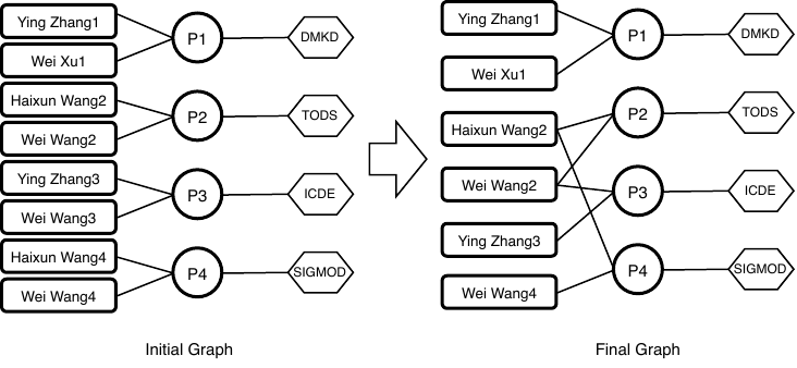
Figure 2. Example heterogeneous multipartite network, such that the left represents the initial scholarly data, and the right represents the final
disambiguation results.
In this section, we first introduce basic notations and then present a formal definition of scholar name disambiguation.
Basic notations. For bibliography data D, each citation record contains title, author names, venue, and publication year. We use the Heterogeneous Information Networks (HINs), which are used widely in complex network analysis [19], [41], to model D. Considering that there are no direct relations among nodes with the same type, we refer to this type of HINs as heterogeneous multipartite networks, which is formally defined as follows.
A heterogeneous multipartite network is an HIN [28] whose node set can be divided into several disjoint sets V 0, V 1,…,V n such that each edge connects a node in V i to another in V j with i≠j. Node sets V 0 , V 1,…,V n are called the parts of the network, and the node types in the same part are identical.
We consider each author reference as a unique author entity initially, then the bibliography data is represented as a 4-part
heterogeneous multipartite network, containing the sets of author nodes (A), paper nodes (P ), venue nodes (V ) and title word nodes
(T ). Fig. 3 shows the network schema [28] of the heterogeneous multipartite network for scholar name disambiguation, where
there are three types of edges in this network, i.e., edges connecting author nodes to paper nodes, paper nodes to venue nodes and
paper nodes to word nodes. We use three matrices to represent the heterogeneous multipartite network  : WAP, WPT and WPV ,
storing author-paper edges, paper-(title) word edges and paper-venue edges in heterogeneous multipartite network ,
respectively.
: WAP, WPT and WPV ,
storing author-paper edges, paper-(title) word edges and paper-venue edges in heterogeneous multipartite network ,
respectively.
We now formalize scholar name disambiguation with the definition of heterogeneous multipartite networks.

Figure 3. Heterogeneous multipartite network for scholar name disambiguation. There are four parts: author (A), paper (P), venue (V ) and title
word (T), and their relationships are labeled with the corresponding adjacency matrices.
Problem statement. Given a heterogeneous multipartite network , the task of scholar name disambiguation is to adjust author
nodes and edges between author and paper nodes, such that for each author a in A, the set of paper nodes Pa connected to a ideally
contains all and only those papers written by author a.
Besides the relationships directly available from the network , we also use the following indirect relationships for the author
similarity computation.
(1) Matrix WAA is for valid coauthorship in , where the entry Wi,jAA is the times that authors i and j collaborates. A coauthor
relation is valid if two authors have different names. Note that, it is possible that a paper is written by more than one author with
the same name. However, we cannot distinguish them without additional information, such as email addresses. In this case, we just
keep an arbitrary author reference and neglect the others. We also dismiss self-coauthorships by setting all Wi,iAA = 0, such that
WAA = WAP × (WAP)T -diag(WAP × (WAP)T).
(2) Matrix WAA2
is for 2-hop coauthorship in , where Wi,jAA2
is the number of valid 2-hop coauthorship paths connecting
authors i and j. To avoid the redundant information, we only consider valid 2-hop coauthorship paths connecting two authors [10].
Specifically, a valid 2-hop coauthorship path in is an APAPA path ai-pi-aj-pj-ak, where ai≠aj, ai≠ak, aj≠ak and
pi≠pj.
(3) Matrices WAN and WAN2 , obtained from matrices WAA and WAA2 , are for (author, coauthor name) relations and (author, 2-hop coauthor name) relations, respectively.
(4) Matrices WAV and WAT are for (author, venue) relations and (author, word) relations, respectively. Wa,vAV is the number of papers that author a publishes in venue v, and Wa,tAT is the times that author a uses word t. That is, WAV = WAP ×WPV and WAT = WAP ×WPT.
(5) Considering that title words or venues may be limited to an author’s publications, we expand these words and venues by considering their similar words and venues. We use matrices WTT and WV V for word-word similarity and venue-venue similarity, respectively. We calculate these two matrices as preprocessing steps before name disambiguation. We present (author, similar word) relations and (author, similar venue) relations with matrices WAST and WASV , respectively, such that WAST = WAT ×WTT and WASV = WAV ×WV V .
Table 1 lists the main symbols and their definitions.
| Symbols | Definitions
|
 | heterogeneous multipartite network |
| A, P , V , T | set of author/paper/venue/word nodes in |
| A(0) | set of author nodes in the initial network |
| N | set of author names in the bibliography data |
| WAP | |
| WPT | adjacency matrices for (A-P), (P-T) and (P-V) |
| WPV | |
| WTT | matrices for word-word similarity |
| WV V | matrices for venue-venue similarity |
| WAA | matrices for coauthorship |
| WAA2 | matrices for 2-hop coauthorship |
| WAN | matrices for (author, coauthor name) relations |
| WAN2 | matrices for (author, 2-hop coauthor name) relations |
| WAV | matrices for (author, venue) relations |
| WASV | matrices for (author, similar venue) relations |
| WAT | matrices for (author, word) relations |
| WAST | matrices for (author, similar word) relations |
| dA, dV , dT | vector for degree of each author/venue/word node |
| dN | vector for number of papers of each name |
| k | vector for estimated author number of each name |
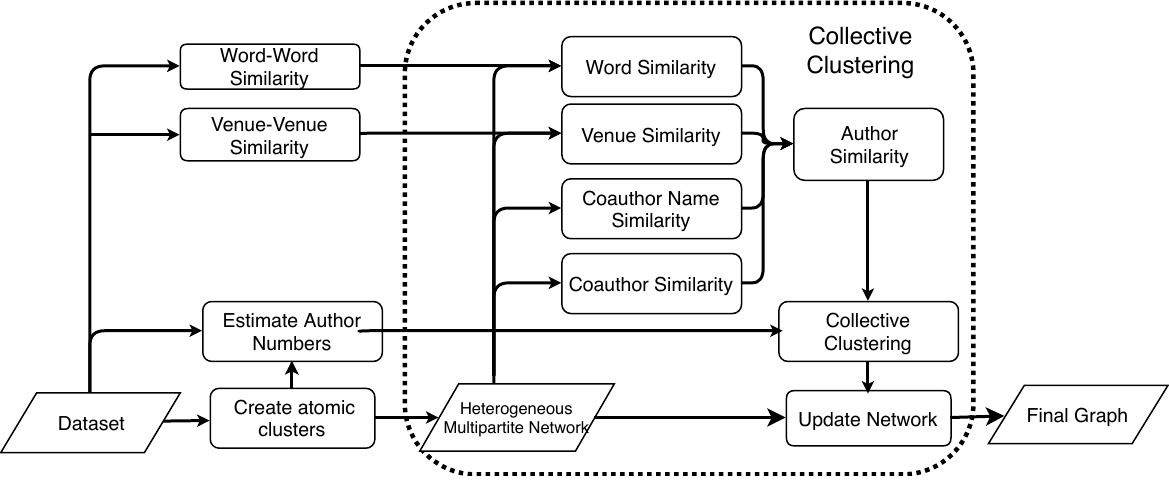
In this section, we introduce our solution framework NDCC, as illustrated in Fig. 4.
(1) Data representation. We represent the bibliography data as a heterogeneous multipartite network, which brings a couple of benefits. First, scholar name disambiguation is formulated with a single network. Specifically, the author nodes in the network are either single author references or atomic clusters (each has several closely related author references) in the beginning. This is a good way to alleviate the error propagation problem caused by ambiguous coauthor names. We disambiguate author names by updating the network, and the final network represents disambiguation results. Second, it is flexible to incorporate extra types of entities such as affiliations and homepages when available.
(2) Similarity measurement. Because of the ambiguity of coauthor names, such as “Ying Zhang” and “Wei Xu” illustrated in Fig. 1, we differentiate coauthors from coauthor names. Then, we determine the author similarity by assembling the similarities from four perspectives (coauthor, venue, title, and coauthor name). It is common that some authors only publish a small number of papers. In this case, venues and title words of their papers are not enough to capture their preferences and research interests, especially in the initial heterogeneous multipartite network, where each author node may only connect to a small number of paper nodes. To alleviate this sparsity problem, we extend the words for authors by considering the words similar to their title words, so do venues. We compute the venue-venue and word-word similarities before name disambiguation begins, as a preprocessing step.
(3) Collective clustering. Obviously, the name disambiguation for one name may influence the others. For example, in Fig. 2, merging of “Haixun Wang2” and “Haixun Wang4” leads to new common coauthor to “Wei Wang2” and “Wei Wang4”, which affects the disambiguation of the name “Wei Wang”. On the other hand, the disambiguation result of “Haixun Wang” is also affected by its coauthors.
Based on the above observation, we propose a bottom-up collective clustering method to deal with scholar name ambiguity. In collective clustering, the disambiguation of one name affects others by changing the structure of the heterogeneous multipartite network. We iteratively select an author name and calculate the pairwise similarities of its author nodes. We then merge the pairs of author nodes with high similarity scores and update the network accordingly. Each name needs to be disambiguated several times until it is fully disambiguated. To determine the stop condition, we estimate the number of authors for each name. A name is considered to be fully disambiguated if the number of its author nodes reaches the estimated number.
4 Author Similarity Measurement
In this section, we present the author similarity measurement. First, we introduce the preprocessing step to deal with the sparsity problem, which is incorporated into author similarities. Then we propose a novel metric to assemble the similarities from four perspectives: coauthors, venues, titles and coauthor names.
As pointed out in Section 3, some authors only connect to a small number of paper nodes, especially in the initial heterogeneous multipartite network. It is hard to make a good judgment for these authors. To deal with this sparsity problem, we introduce word-word and venue-venue similarities to expand the limited information.
(1) Word-word similarity. The title is an important feature to calculate pairwise similarities of authors for name disambiguation. The traditional unigram model treats each word separately and neglects their correlations. It is likely that two titles, which do not share common words, are correlated. For example, one title contains the word “hardware” and the other contains the word “circuit”. Both are related to computer hardware. In this case, the traditional unigram model returns a low similarity score. In [17], [18], the string level or character level tolerance is used when comparing two titles. However, these methods cannot capture the semantic relation between two words either.
We propose to use Word2vec [24], which is an effective word embedding method, to capture the semantic correlations between words. It takes a text corpus as input and maps each word in the text corpus to a vector in a low dimensional space. First, we normalize all titles using NLTK [8] by turning them into lowercase, removing punctuation, tokenizing and removing stop words. All normalized titles are used as the training text corpus for Word2vec. Then the cosine similarity of word vectors is used as the word-word similarity, which is stored in a matrix denoted by WTT. We keep the pairs whose similarity scores are larger than a threshold σt, and disregards the others by setting the similarity scores to zeroes.
(2) Venue-venue similarity. We expand venues for each author, based on an observation that two venues are similar if a large portion of authors both publish papers in these two venues. For example, “SIGMOD” and “VLDB” are both top database conferences, and many authors publish papers in both venues. Hence, “SIGMOD” and “VLDB” are two similar venues. Based on this observation, we propose to use the Jaccard index of authors to measure venue-venue similarity. Formally, given two venues i and j, Ni and Nj represent the sets of author names who publish at least one paper in i and j, respectively. The similarity between venue i and j is defined as

Here we only keep venue pairs with their similarity scores larger a threshold σv, and neglect the others by setting their scores to 0 in WV V .
4.2 Author Similarity Assembling
The author similarity is assembled by four similarities (coauthor, venue, title, and coauthor name). Given two authors i and j with the same name n, inspired by [18], we consider each pair and define the author similarity as:
sim =  , , | (1) |
where x,y ∈{n,t,v,a} and sima,simn,simt,simv are coauthor, coauthor name, title and venue similarities, respectively. We omit (i,j) in Eq. (1) as well as equations in the sequel for simplicity.
We argue that two authors are likely to be the same person if they are similar in at least two aspects. For example, in Fig. 2, “Haixun Wang2” and “Haixun Wang4” are similar in terms of coauthor names and venues, so it is likely that they are the same person. On the other hand, in Fig. 1, although these two “Wei Xu” are similar in the perspective of coauthor name, they are not similar in other perspectives. Thus, they are unlikely to be the same author.
Intuitively, the more two authors share the same related entities (coauthors, title words, venues, and coauthor names), the more similar they are. Histogram intersection kernel is a common way to measure this similarity between two histograms [29]. Besides, similar to IDF [15], weights of different entities should be normalized by their frequencies. For example, if a coauthor publishes a lot of papers, then it should be considered as a weak evidence comparing to those who only publish one or two papers. Since productive authors are believed to be experts connecting different communities, they likely collaborate with two or more authors with the same name. For instance, “Haixun Wang” in WeWork has over 100 papers, and collaborates both with “Wei Wang” in UCLA and “Wei Wang” in UNSW. From the title perspective, common words, such as “approach” and “system” are less representative comparing to uncommon words like “disambiguation” and “collective”. So we differentiate weights of words by assuming that the more frequently a word appears in titles, the less important the word is as evidences. The other two perspectives, i.e., venues and coauthor names, follow similar principles.
(1) Coauthor similarity. Based on the above observations, we use the normalized histogram intersection kernel to calculate the coauthor similarity sima, defined as
| sima = | ∑
k min(Wi,kAA,W
j,kAA) + t(n){∑
k min(Wi,kAA,W
j,kAA) + t(n){∑
k min(Wi,kAA,W
j,kAA2) min(Wi,kAA,W
j,kAA2) | ||
+ ∑
k min(Wi,kAA2,W
j,kAA))}, min(Wi,kAA2,W
j,kAA))}, | (2) |
where t(n) =  . Here dkA is the number of papers written by author k, which serves the normalization
factor, and θ is a threshold determining whether to use multi-hop coauthorships. The first part of the right side of
Eq. (2) measures the similarity between coauthors of i and j. The second considers multi-hop coauthors. Comparing
with (1-hop) coauthor, multi-hop coauthors are less evidential. We notice that for names with high ambiguities,
such as “Wei Wang”, using weak evidential features like multi-hop coauthors may introduce errors and decrease
the accuracy performance. Thus, for these names, we neglect the multi-hop coauthorship, and only use the first
part.
. Here dkA is the number of papers written by author k, which serves the normalization
factor, and θ is a threshold determining whether to use multi-hop coauthorships. The first part of the right side of
Eq. (2) measures the similarity between coauthors of i and j. The second considers multi-hop coauthors. Comparing
with (1-hop) coauthor, multi-hop coauthors are less evidential. We notice that for names with high ambiguities,
such as “Wei Wang”, using weak evidential features like multi-hop coauthors may introduce errors and decrease
the accuracy performance. Thus, for these names, we neglect the multi-hop coauthorship, and only use the first
part.
The other similarity scores, i.e., Coauthor name, title, and venue similarities, are defined similarly.
(2) Coauthor name similarity.
| simn = | ∑
m min(Wi,mAN,W
j,mAN) + t(n){∑
m min(Wi,mAN,W
j,mAN) + t(n){∑
m min(Wi,mAN,W
j,mAN2) min(Wi,mAN,W
j,mAN2) | ||
+ ∑
m min(Wi,mAN2,W
j,mAN)}, min(Wi,mAN2,W
j,mAN)}, | (3) |
where t(n) is the same as the one in Eq. (2), and dmN is the number of papers written by authors with name m.
(3) Title similarity.
| simt = | ∑
t min(Wi,tAT,W
j,tAT) + {∑
t min(Wi,tAT,W
j,tAT) + {∑
t min(Wi,tAT,W
j,tAST) min(Wi,tAT,W
j,tAST) | ||
+ ∑
t min(Wi,tAST,W
j,tAT)}, min(Wi,tAST,W
j,tAT)}, | (4) |
where dtT is the number of papers containing the word t, and we use the bag-of-words model to represent titles. The first part of the right side of Eq. (4) measures the similarity between words both author i and j used in their paper titles. The second part takes similar words into consideration.
(3) Venue similarity.
| simv = | ∑
v min(Wi,vAV ,W
j,vAV ) + {∑
v min(Wi,vAV ,W
j,vAV ) + {∑
v min(Wi,vAV ,W
j,vASV ) min(Wi,vAV ,W
j,vASV ) | ||
+ ∑
v min(Wi,vASV ,W
j,vAV )}, min(Wi,vASV ,W
j,vAV )}, | (5) |
where dvV is the number of papers published in venue v. The first part of the right side of Eq. (5) measures the similarity between venues where both author i and j publish papers in. The second part considers similar venues.
In this section, we first introduce the collective clustering algorithm with speeding-up strategies for scholar name disambiguation. Our method follows a bottom-up fashion. In the beginning, each author reference is considered as an individual author entity. Different from the density-based clustering method, such as DBSCAN, where distances between points (or nodes) remain unchanged, our collective clustering method dynamically updates similarities during the disambiguation process. We also analyze its convergence rate as well as time and space complexities of NDCC.
For scholar name disambiguation, some author references can be easily clustered together. For example, papers “Clustering by pattern similarity in large data sets”, and “Improving performance of bicluster discovery in a large data set” share the same author names “Jiong Yang”, “Wei Wang” and “Haixun Wang”. There is a strong probability that these two “Wei Wang” are the same person because they have two identical coauthor names. These two author references form an atomic cluster. Generating atomic clusters as the bootstrap can reduce the size of the initial network, and improve the efficiency. Bootstrap strategies, such as rule based methods, are used widely in the previous name disambiguation methods [7], [30], [35]. Note that, using improper rules may include false positive pairs and impair the accuracy performance, such as the example shown in Fig. 1. Thus, we adopt a highly restrictive rule to generate atomic clusters to significantly alleviate this problem. Inspired by the above observations, two author references are assigned to the same atomic clusters if they share at least two coauthor names.
As mentioned in the solution framework in Section 3, the estimated number of authors for each name is used as the stop condition in collective clustering. Specifically, a name is considered as fully disambiguated if the number of authors of this name reaches the estimated one. Inspired by name ambiguity estimation in the paper [18], we introduce a statistical method, which is based on the statistics of author names in the bibliography data.
In most cases, a name consist of a fixed number of components. For instance, an English name has three parts: the first name,
middle name and last name, and a Chinese name consists of the first name and last name. We assume that these parts are chosen
independently from different multinomial distributions, and the probability of a full name is the joint probability of its components
[18]. Here we use the two-component names as an example to explain the main idea. Given a name n, its first name and
last name are denoted by F(n) and L(n), which are independently drawn from multinomial distributions MultiF
and MultiL, respectively. The probability of an author with name n is Pr(n) = MultiF(F(n)) × MultiL(L(n)).
Then, the number of authors with name n is kn = Pr(n)∑
e∈N e, where
  e is the number of authors with name e,
and ∑
e∈N
e is the number of authors with name e,
and ∑
e∈N e is the total number of authors in the bibliography data. Since
  e is unknown, we use its estimate ke
instead.
e is unknown, we use its estimate ke
instead.
Parameters of MultiF are estimated by the maximum likelihood estimation. Specifically, πf, the probability of a first
name f appears, is estimated by πf =  . So do parameters in MultiL. We use an EM-like method to
update k and parameters in MultiF and MultiL iteratively. Specifically, in the beginning, we set kn = 1 for each
name n. At each expectation step, we fix parameters in MultiF and MultiL, and update k. During iterations, it is
possible that kn < 1 or kn > |An(0)|, where |An(0)| is the number of atomic author clusters of name n. In this case,
we round kn to 1 if kn < 1, and |An(0)| for the second case. At each maximization step, we update parameters
in MultiF and MultiL with the k fixed. Expectation and maximization steps are alternatively repeated until k
converges.
. So do parameters in MultiL. We use an EM-like method to
update k and parameters in MultiF and MultiL iteratively. Specifically, in the beginning, we set kn = 1 for each
name n. At each expectation step, we fix parameters in MultiF and MultiL, and update k. During iterations, it is
possible that kn < 1 or kn > |An(0)|, where |An(0)| is the number of atomic author clusters of name n. In this case,
we round kn to 1 if kn < 1, and |An(0)| for the second case. At each maximization step, we update parameters
in MultiF and MultiL with the k fixed. Expectation and maximization steps are alternatively repeated until k
converges.
 1Use
BFS
to
calculate
WAA,
WAA2
,
WAT,
WAST,
WAV ,
WASV ;
2Initialize
an
empty
queue
que;
3foreach author
name
n do
4
5
6An
←
the
list
of
authors
with
name
n;
7if |An|> 1 then
8
9
10que.push(n);
11while
que
is
not
empty do
12
13
14n ←que.pop();
15An
←
the
list
of
authors
with
name
n;
16if |An|≤kn then
17
18
19Continue
20K ←⌈
1Use
BFS
to
calculate
WAA,
WAA2
,
WAT,
WAST,
WAV ,
WASV ;
2Initialize
an
empty
queue
que;
3foreach author
name
n do
4
5
6An
←
the
list
of
authors
with
name
n;
7if |An|> 1 then
8
9
10que.push(n);
11while
que
is
not
empty do
12
13
14n ←que.pop();
15An
←
the
list
of
authors
with
name
n;
16if |An|≤kn then
17
18
19Continue
20K ←⌈ ⌉;
21Calculate
pairwise
similarities
of
authors
in
An
with
Eq.
(1);
22t ←
the
K-th
largest
pairwise
similarity
score;
23Merge
author
pairs
whose
similarity
scores
are
no
less
than
t;
24Update
the
author-paper
matrix
WAP
according
to
Eq.
(7);
25Update
WAA,
WAA2
,
WAT,
WAST,
WAV
and
WASV
according
to
Eq.
(8,
9,
10);
26que.push(n);
27Return
WAP.
_______________________________________________________________________________________________________________________________________________________________________________________________________________________________
⌉;
21Calculate
pairwise
similarities
of
authors
in
An
with
Eq.
(1);
22t ←
the
K-th
largest
pairwise
similarity
score;
23Merge
author
pairs
whose
similarity
scores
are
no
less
than
t;
24Update
the
author-paper
matrix
WAP
according
to
Eq.
(7);
25Update
WAA,
WAA2
,
WAT,
WAST,
WAV
and
WASV
according
to
Eq.
(8,
9,
10);
26que.push(n);
27Return
WAP.
_______________________________________________________________________________________________________________________________________________________________________________________________________________________________
Given an initial heterogeneous multipartite network , which is created directly from the bibliography data with
bootstrap, as well as the preprocessing results: WV V , WTT and k, collective clustering returns the final author-paper
matrix, where each author node represents an author entity in the real world, and connects to all its paper nodes
only.
In collective clustering, disambiguation of one name affects the others by updating the structure of the heterogeneous
multipartite network . In each iteration, we focus on a name n, instead of directly employing hierarchical clustering methods to
merge the author nodes with name n, until the number reaches kn. We merge the top K pairs with the highest similarity
scores. Here we choose K as the half of the difference between the current author number and the estimated one.
Formally,
| (6) |
where |An| is the number of authors with name n in this iteration. Our framework also supports other choices of K, and we leave this part as future work. Each name is disambiguated iteratively until it is fully disambiguated, i.e., the number of its authors reaches the estimated number. The final network is the disambiguation result.
Observe that it is time-consuming to re-calculate matrices such as WAA and WAA2
in each iteration when network is updated
for the merging of author nodes, we introduce speeding-up strategies for the computation. We calculate and store those matrices
such as WAA and WAA2
as a preprocessing step before iterations, and update them inside iterations. Considering the sparsity and
dynamics of matrices, we use lists of treemaps to store WAA, WAA2
, WAT, WAST, WAV and WASV . Specifically,
for each author name, we maintain a list of its author nodes. Each author node contains six treemaps to store the
corresponding rows in these metrics, respectively. Considering that the author name is just an attribute attached
to the author node, we do not store WAN and WAN2
, as they can be extracted directly from WAA and WAA2
,
respectively.
We now explain the detail of our collective clustering. Algorithm 1 shows its overall process. First, it uses breadth-first search to
calculate all the metrics such as WAA, WAA2
from the input (line 1), and then uses a queue que to store the names to be
disambiguated, which is initiated by pushing all names in the bibliography data, except those with only one paper (lines 2-6). Our
method iteratively disambiguates author names (lines 7-18). While que is not empty, it pops out a name from que, denoted by n (line
8), and assigns An the list of author nodes with name n (line 9). If the size of An is no larger than kn, then the name n is believed to
be fully disambiguated. In this case, it just continues to deal with the next name (lines 10-11). Otherwise, it calculates the number of
pairs to be merged in this iteration by Eq. (6), denoted by K (line 12). It then calculates pairwise author similarity scores in An,
and finds K-th largest score t by using a K-size minimum heap (lines 13-14). Then it merges author pairs whose
similarity scores are no less than t, and updates the network (equally, the matrix WAP) accordingly (lines 15-16). It
also needs to update WAA etc. (line 17). Then it pushes n into que, and waits for disambiguation results of the
remaining names (line 18). After all names have been processed, it finally returns the disambiguation result WAP (line
19).
Next, we present the updating rules for matrices WAA, WAA2 , WAT, WAST, WAV and WASV . Given authors i and j to be merged, without loss of generality, we assume that j is merged to i, and the updated i is denoted by î.
By the definition, the author-paper matrix WAP is updated as follows.
| (7) |
, where a hat denotes the updated matrix.
The author-author matrix WAA is updated as follows.
| (8) |
Correctness of Eq. (8): Correctness of Eq. (8) can be proved by combining the definition of WAA and Eq. (7). □
Considering that merging of two author nodes incorporates new 2-hop coauthorships, matrix WAA2 is updated as follows.
| (9) |
Correctness of Eq. (9): We denote the set of valid coauthor paths and valid 2-hop coauthor paths connecting author k and l by  k,l
and k,l2, respectively. We use a ∈ p if path p contains author a, and use hats to represent the updated sets. Then Wk,lAA = |k,l|
and Wk,lAA2
= |k,l2|.
k,l
and k,l2, respectively. We use a ∈ p if path p contains author a, and use hats to represent the updated sets. Then Wk,lAA = |k,l|
and Wk,lAA2
= |k,l2|.
By the definition of the valid 2-hop coauthor path, if k = l, we have  k,lAA2
= |
k,lAA2
= | k,l2| = 0. Next, we discuss the other cases
where k≠l.
k,l2| = 0. Next, we discuss the other cases
where k≠l.
(1) If k = î, then

(2) If l = î, then

(3) Otherwise

Similarly, we update  AV ,
AV ,  ASV ,
ASV ,  AT and
  AST by
| (10) |
Correctness of Eq. (10): Since WPV is static, we can prove the correctness of updating WAV by combining definition of WAV and updating rules of WAP. Considering WV V is also static, we can prove the correctness of updating rule for WASV by definition of WASV and updating rules of WAV . Similarly, we can prove the correctness of updating rules for WAT and WAST. □
After merging author j to author i, we delete the corresponding rows and columns from the updated matrices.
5.5 Convergence and Complexity Analyses
We denote the set of author nodes in the initial heterogeneous multipartite network by A(0). It is easy to find that the size of A is non-increasing. Thus, it is obvious that collective clustering converges.
We denote the largest number of papers written by the authors with the same name as ℓ, and then prove the bound of the number of iterations as the following.
Theorem 1 (Iteration number). The iteration number of collective clustering is no more than |N|(log(ℓ) + 2).
Proof. We denote the iteration number by TN and the number of iterations dealing with name n by Tn. Then TN = ∑
n∈NTn. We
also denote the number of authors with name n after the i-th iteration dealing with n by |An(i)|. Initially, |An(0)| is the number of
atomic authors with name n. According to Eq. (6), An(i+1) = |An(i)|-⌈ ⌉. Then we have |An(i)| = ⌊
 ⌋ + kn and
Tn = ⌈log(|An(0)|-kn)⌉ + 1. Finally, we have
⌋ + kn and
Tn = ⌈log(|An(0)|-kn)⌉ + 1. Finally, we have
The time complexity of collective clustering is O(ℓ2 log(ℓ)(H + |A(0)|log(ℓ))), where H = ∑
n(|An(0)|2) is the number of atomic
author pairs sharing the same names. The space complexity is O(|A(0)|ℓ2). More specifically, We use the same notations as the proof
of Theorem 1. We assume that each paper has no more than α keywords in its title, and has no more than β authors. The time
complexity of creating initial matrices is O(|A(0)|(ℓ2β2 log(ℓβ) + ℓα log(ℓα))). Since elements in treemaps are sorted, we only need
to traverse the corresponding treemaps to calculate the author similarity, which takes linear time w.r.t. the sizes of treemaps. So it
takes O(ℓ2β2 + ℓα) time to calculate the similarity of two authors. For each pair of author nodes to be merged, based on Eq. (8, 9,
10), it takes O(ℓ2β log(ℓβ) + ℓα log(ℓα)) time to update matrices as well as . In most cases, a paper contains no more than 10
authors, and no more than 10 keywords. Treating α and β as constants, the time complexities of calculating the
similarity of two authors and merging two author nodes are O(ℓ2) and O(ℓ2 log(ℓ)), respectively. From Theorem 1,
each name n is disambiguated ⌈log(|An(0)|-kn)⌉ + 1 times. In the i-th iteration dealing with name n, it takes
O(|An(i)|2 log(|An(i)|)) time to find the K-th largest similarity score. Putting these together, the time complexity of
collective clustering is O(ℓ2 log(ℓ)(H + |A(0)|log(ℓ))), where H = ∑
n(|An(0)|2) is the number of atomic author
pairs sharing the same names. It takes O(|A(0)| + |P|(1 + β + α)) space to store and preprocessing results, and
O(|A(0)|(ℓ2β2 + ℓα)) space to store the other matrices. By considering α and β as constants, the space complexity is
O(|A(0)|ℓ2).
In this section, we present an extensive experimental study of NDCC. Using three real datasets, we conduct four sets of experiments to evaluate (1) the effectiveness and efficiency of NDCC versus state-of-the-art methods CE [7], GHOST [10], CSLR [18], MIX [17], and AM [42], (2) the effectiveness of author number estimation, (3) effects of important components in NDCC, and (4) the impacts of parameters on accuracy and efficiency.
We first introduce our experimental settings.
Datasets. We use three commonly used real-life datasets AMiner (http://www. aminer.org) [30], [31], [32], [35] , ACM (http://dl.acm.org) [35] and DBLP (http://dblp.uni-trier.de) [18] for scholar name disambiguation. Different from previous works that use small size subsets, we build datasets from the whole public available meta-data files directly. The statistics of these datasets are listed in Table 2.
| Name | |P| | |T| | |V | | |N|
|
| AMiner | 1,397,240 | 233,503 | 16,442 | 1,062,896 |
| ACM | 2,381,719 | 327,287 | 273,274 | 2,002,754 |
| DBLP | 3,566,329 | 251,429 | 12,486 | 1,871,439 |
The test set comes from https://aminer.org/disambiguation, which is commonly used in name disambiguation tasks [30], [35]. It contains 6,730 labeled papers of 110 author names. We compare the labeled papers with each dataset and use their overlapped ones as the corresponding testing dataset. We use the Macro-F1 score to evaluate the effectiveness.
Comparison algorithms. Although NDCC can be easily extended to incorporate other information like affiliations, paper abstracts, homepages, and email addresses, the datasets that we use only contain citation information, like many other digital libraries. Thus, we dismiss baselines relying on these external features [30], [35], [36]. Besides, some methods require the number of authors for each name [36], [37], which is unavailable in practice. Thus, we compare NDCC with the following state-of-the-art methods, which can determine the author numbers automatically and use citation information only.
(1) CE [7] is a collective entity resolution method for relational data. Its similarity function considers both attributes and relational information, and a greedy agglomerative clustering method is used to merge the most similar clusters.
(2) GHOST [10] is a graph-based method employing coauthorship only. Its similarity function considers both quantity and quality (length) of paths, and an affinity propagation clustering method is used to generate clusters of author references of the focused name.
(3) CSLR [18] first groups the author references based on coauthorships to generate initial clusters. Then these clusters are merged by venue-based and title-based similarities.
(4) MIX [17] is a supervised method. Random forests are used to calculate pairwise distances, and DBSCAN is used to group the author references. For effectiveness evaluation, we randomly choose 5 (other) labeled names as the training set for each author name to be disambiguated. For efficiency evaluation, we randomly choose 5 labeled names to train the model and use the others for testing.
(5) AM [42] is the method deployed in AMiner to tackle the name disambiguation. A representation learning method is used to include global and local information. An end-to-end method is proposed to estimate author numbers. We train the model with 500 labeled author names reported in their paper. For a fair comparison, we dismiss non-citation features, including abstracts and affiliations.
| Name | AMiner | ACM | DBLP | |||||||||||||||
| CE | GHOST | CSLR | MIX | AM | NDCC | CE | GHOST | CSLR | MIX | AM | NDCC | CE | GHOST | CSLR | MIX | AM | NDCC | |
| Wen Gao | 64.0 | 46.1 | 87.3 | 8.8 | 83.6 | 91.8 | 90.4 | 48.9 | 90.7 | 8.1 | 89.3 | 96.2 | 91.9 | 79.7 | 95.4 | 3.8 | 73.0 | 96.3 |
| Lei Wang | 41.8 | 20.3 | 53.2 | 39.0 | 21.2 | 59.7 | 7.8 | 24.0 | 23.8 | 48.7 | 26.1 | 55.1 | 14.4 | 15.2 | 57.2 | 29.9 | 18.7 | 77.4 |
| David E. Goldberg | 85.2 | 73.0 | 81.0 | 7.6 | 96.6 | 98.3 | 82.9 | 74.5 | 91.9 | 8.1 | 93.8 | 98.5 | 79.3 | 73.9 | 97.1 | 5.7 | 100.0 | 100.0 |
| Yu Zhang | 52.8 | 30.9 | 53.2 | 50.0 | 34.1 | 67.2 | 10.7 | 25.2 | 41.4 | 48.4 | 28.3 | 68.8 | 16.6 | 15.7 | 68.2 | 33.3 | 31.5 | 57.3 |
| Jing Zhang | 43.7 | 33.1 | 56.3 | 54.3 | 31.7 | 50.3 | 14.0 | 22.2 | 53.0 | 56.9 | 33.6 | 67.4 | 20.7 | 12.7 | 63.7 | 46.3 | 22.6 | 61.8 |
| Lei Chen | 51.8 | 36.6 | 76.0 | 13.1 | 28.1 | 72.4 | 53.5 | 39.4 | 78.1 | 12.1 | 26.4 | 72.2 | 59.5 | 46.1 | 75.1 | 8.0 | 38.1 | 70.1 |
| Yang Wang | 36.4 | 40.0 | 29.6 | 18.6 | 19.1 | 42.6 | 19.4 | 36.4 | 34.7 | 20.3 | 30.0 | 34.9 | 38.1 | 62.8 | 43.5 | 23.7 | 22.6 | 44.1 |
| Bing Liu | 56.3 | 40.8 | 61.0 | 6.3 | 53.1 | 62.2 | 47.3 | 49.1 | 70.3 | 5.3 | 82.6 | 73.6 | 61.6 | 42.7 | 68.9 | 5.0 | 67.9 | 73.1 |
| Hao Wang | 35.8 | 41.5 | 48.1 | 43.7 | 33.8 | 59.4 | 13.6 | 39.4 | 52.3 | 62.9 | 35.1 | 56.5 | 20.6 | 14.4 | 48.4 | 37.9 | 43.0 | 57.3 |
| Gang Chen | 43.4 | 46.5 | 57.7 | 46.7 | 20.7 | 59.7 | 44.7 | 59.4 | 50.1 | 44.6 | 22.4 | 62.7 | 56.7 | 46.1 | 61.1 | 17.9 | 37.5 | 66.1 |
| # Top Names | AMiner | ACM | DBLP | |||||||||||||||
| CE | GHOST | CSLR | MIX | AM | NDCC | CE | GHOST | CSLR | MIX | AM | NDCC | CE | GHOST | CSLR | MIX | AM | NDCC | |
| 10 | 51.1 | 40.9 | 60.3 | 28.8 | 45.5 | 66.4 | 38.4 | 41.9 | 58.6 | 31.5 | 46.8 | 68.6 | 45.9 | 40.9 | 67.9 | 21.1 | 45.4 | 73.1 |
| 20 | 48.8 | 44.8 | 60.7 | 24.5 | 45.0 | 67.7 | 34.1 | 43.2 | 56.2 | 32.1 | 45.1 | 71.8 | 45.6 | 42.6 | 70.1 | 22.3 | 47.5 | 71.9 |
| 30 | 49.0 | 50.7 | 56.8 | 24.4 | 52.0 | 70.8 | 35.6 | 49.1 | 56.4 | 31.6 | 54.6 | 72.4 | 52.6 | 51.8 | 71.1 | 21.9 | 54.8 | 77.7 |
| 40 | 53.0 | 52.0 | 57.6 | 27.9 | 49.8 | 70.5 | 40.0 | 51.8 | 57.6 | 35.0 | 54.5 | 72.1 | 56.3 | 53.3 | 72.0 | 25.6 | 57.7 | 79.7 |
| 50 | 52.6 | 51.9 | 58.2 | 27.9 | 51.5 | 72.0 | 42.7 | 52.8 | 58.3 | 35.2 | 55.7 | 75.0 | 58.4 | 54.6 | 73.9 | 26.2 | 61.3 | 79.9 |
| 60 | 54.9 | 51.2 | 58.4 | 30.0 | 52.0 | 73.0 | 46.5 | 53.3 | 60.0 | 35.8 | 57.3 | 76.0 | 61.4 | 53.4 | 74.1 | 27.3 | 63.7 | 79.5 |
| 70 | 57.3 | 52.1 | 58.3 | 30.0 | 52.7 | 74.5 | 49.2 | 52.9 | 60.2 | 37.4 | 58.2 | 76.9 | 63.9 | 54.6 | 74.4 | 28.3 | 66.3 | 80.9 |
| 80 | 58.3 | 52.4 | 58.4 | 30.4 | 54.3 | 74.6 | 51.1 | 53.4 | 61.2 | 38.6 | 60.2 | 77.2 | 66.7 | 56.7 | 73.9 | 28.6 | 68.3 | 81.0 |
| 90 | 57.6 | 52.2 | 57.9 | 30.1 | 54.9 | 75.5 | 51.2 | 52.8 | 60.6 | 38.7 | 61.5 | 76.9 | 66.9 | 56.8 | 73.0 | 29.5 | 69.7 | 80.9 |
| 100 | 58.0 | 52.7 | 59.3 | 30.6 | 54.7 | 76.0 | 52.1 | 53.2 | 61.8 | 40.0 | 62.5 | 77.5 | 67.7 | 57.5 | 72.3 | 30.4 | 70.9 | 80.8 |
Implementation. In NDCC, the threshold for word-word similarity σt is set to 0.75, the threshold for venue-venue similarity σv is set to 0.02, and the threshold for using weak evidence θ is set to 20. For the other methods, all parameters are set to their default values. All experiments are conducted on a machine with 2 Intel Xeon E5-2630 2.4GHz CPUs and 64 GB of Memory, running 64-bit windows 7 professional system. Each experiment is repeated 5 times, and the average is reported here.
We next present our findings.
Exp-1: Performance comparison with baselines. In the first set of experiments, we evaluate the effectiveness and efficiency of NDCC against CE, GHOST, CSLR, MIX and AM.
Exp-1.1: Accuracy performance comparison. The accuracy results for all methods in three datasets are shown in Table 3 and Table 4. In practice, the disambiguation of a name is much challenging if a large number of papers are written by authors with the same name. Thus, we rank the author names in the test set based on paper numbers and list the Macro-F1 scores of the top 10 names with the largest number of papers in Table 3. The number of real authors for each name and the corresponding total number of publications are listed in Table 5. To demonstrate the effeteness of NDCC on the whole dataset, we vary M from 10 to 100 and report results of the top M names in Table 4. For each row, the top performer is highlighted in the bold font.
We observe that NDCC consistently outperforms baselines. NDCC achieves the best performances on 8, 6 and 6 out of 10 names listed in Table 3 in AMiner, ACM and DBLP, respectively. With the top 100 names as the testing dataset, NDCC improves the Macro-F1 over (CE, GHOST, CSLR, MIX, AM) by (17.87%, 23.25%,16.65%,45.39%, 21.24%) on AMiner, (25.36%, 24.26%, 14.16%, 37.46%, 14.96%) on ACM, and (13.11%, 23.31%, 8.47%, 50.37%, 9.86%) on DBLP, on average, respectively. MIX adopts random forests to learn pairwise similarities, which works well when many features are available, such as abstract, and affiliation [17]. While, in this study, we address the scholarly name disambiguation problem in a more challenging setting, where only basic citation features are available. We observe that in this setting, a large number of pairwise similarities are 0. As a result, in most cases, MIX achieves high precision scores with very low recall scores, leading to its low F1 scores. GHOST only uses coauthorships, which explains its unsatisfactory accuracy performance. Besides, 3 and 4-hop coauthorships used in GHOST are weak evidences. The ambiguity of (multi-hop) coauthors further harms the accuracy results. CE neglects the venue-venue and word-word similarities, which leads to its low F1 scores. CSLR is a single name disambiguation method that also considers the similarity between venues and words to alleviate the problem caused by limited information. NDCC outperforms it by (28.07%, 25.32% and 11.71%) on (AMiner, ACM, DBLP), which justifies the advantage of collective clustering. Without external information, AM still achieves relatively good results, compared with other baselines. However, this method neglects 2-hop coauthors, which are important features when only citation information is available.
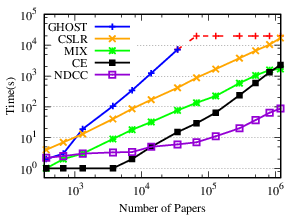
Exp-1.2: Efficiency performance comparison. Among the chosen baselines, only CE and GHOST analyze the time complexity [7], [10]. The time complexity of CE is O(|A(0)|k log |A(0)|), where |A(0)| is the number of atomic authors, and k is largest number of buckets that a buckets connects to [7]. It is difficult to exactly compare CE and our method because of k, which is unique to the method. The time complexity of GHOST is O(Nℓ2), where N is the number of names to be disambiguated, and ℓ is the largest number of papers written by authors with the same name. Although it is theoretically efficient, as a single name disambiguation method, GHOST has to extract a subgraph for each name, which is time consuming in practice.
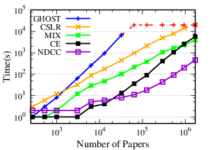
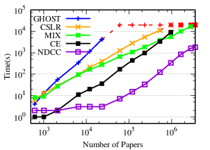
To empirically evaluate the efficiency of NDCC, we extract several subsets from AMiner (ACM, DBLP) with different sizes by author names. First, we generate several subsets of author names from AMiner ( ACM, DBLP), with sizes ranging from 50 to 1M (2M and 1.8M on ACM and DBLP, respectively). To maintain the consistency among these sets, we make sure that smaller sets are subsets of the bigger ones. For each set of author names, we extract all papers written by authors in this set to generate the corresponding subset. In this way, we make sure that the generated subsets are dense. Although AM is deployed with thousands of millions of papers, it is not efficient to compute the clustering from scratch due to the local linkage learning and IO overhead [42]. Indeed, this method even cannot disambiguate all names in the smallest dataset AMiner within 12 hours. Thus, its running time is not reported here.
| Name | #Authors | # Papers | AMiner | ACM | DBLP |
| Wen Gao | 10 | 461 | 12 | 12 | 21 |
| Lei Wang | 106 | 289 | 91 | 98 | 122 |
| David E. Goldberg | 3 | 211 | 4 | 4 | 18 |
| Yu Zhang | 65 | 209 | 62 | 87 | 99 |
| Jing Zhang | 76 | 198 | 61 | 74 | 93 |
| Lei Chen | 35 | 179 | 39 | 34 | 52 |
| Yang Wang | 48 | 177 | 52 | 59 | 68 |
| Bing Liu | 16 | 171 | 32 | 29 | 23 |
| Hao Wang | 46 | 165 | 48 | 55 | 73 |
| Gang Chen | 40 | 163 | 35 | 44 | 57 |
The results show that NDCC is more efficient than the baseline methods. (a) NDCC is (18, 195, 19) times faster than (CE, CSLR and MIX) on AMiner, (15, 8) times faster than (CE, MIX) on ACM, 10 times faster than MIX on DBLP, on average, respectively. (b) While GHOST on (AMiner, ACM, DBLP), CSLR on (ACM, DBLP) and CE on DBLP could not finish in 6 hours, NDCC could finish on (AMiner, ACM, DBLP) in (98, 543, 2106) seconds, respectively.
Exp-2: Effectiveness of estimating author numbers. In the second set of experiments, we evaluate the effectiveness of NDCC in
estimating author numbers. We note that the test dataset does not cover all authors in the datasets, and only part of the authors
are labeled. For example, there are over 120 authors with the name “Lei Wang” in DBLP, but only 106 of them are
labeled. Thus, We cannot evaluate the estimation method directly by comparing the estimated author numbers with
labeled authors. Instead, given a name, we compare the number of clusters of the labeled papers with the number
of labeled authors to verify the effectiveness of the proposed estimating method. We list the results of the top 10
names in the test set in Table 5. We find that, in most cases, our method achieves reasonable estimating results:
 ∈ (0.5,2). Besides, the numbers of detected authors are usually larger than the true values. The reason is
that authors may change their affiliations and research interests at the same time. In this case, it is hard for name
disambiguation methods to tell whether papers published in two periods are written by the same person with limited
information.
∈ (0.5,2). Besides, the numbers of detected authors are usually larger than the true values. The reason is
that authors may change their affiliations and research interests at the same time. In this case, it is hard for name
disambiguation methods to tell whether papers published in two periods are written by the same person with limited
information.
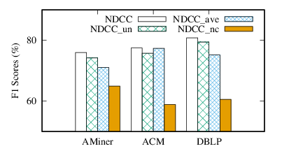
Exp-3: Insight of effectiveness. In the third set of experiments, we analyze the effectiveness of each step in NDCC by comparing with its variants. Specifically, we introduce word-word and venue-venue similarities to alleviate the sparsity problem, a new metric to compute the author similarity by considering different aspects, a statistical method to accurately estimate author numbers, and a collective approach to clustering. Since we have two parameters, σt and σv, to control the usage of word-word similarities and venue-venue similarities, we left the evaluations of these two steps in the parameter studies. We adopt three variants, NDCC_un, NDCC_ave, and NDCC_nc to evaluate effects of author similarity computation, author number estimation, and collective clustering, respectively. With the top 100 author names, we compare these variants with NDCC in three datasets. The comparison results are shown in Fig. 6.
Exp-3.1: Effectiveness of author similarity computation. We consider four features to determine the author similarity. Normalized histogram intersection kernels are adopted, which consider the importance of each word, venue, coauthor, and coauthor name. To demonstrate its effectiveness, we compare NDCC with its variant, denoted by NDCC_un, which adopts (unnormalized) histogram intersection kernels. As shown in Fig. 6, normalization in author similarity computations improves the F1 scores by (4.43%, 2.34%, and 1.69%) on three datasets, respectively.
Exp-3.2: Effectiveness of author number estimation. To demonstrate the effects of author number estimation, we compare NDCC with its variant NDCC_ave, which adopts a simple way to estimate the author numbers. From the test set, we know that on average, each author writes r = 4.87 papers. NDCC_ave estimates the number of authors for each name n with # authors = (# papers written by name n)/r. From Fig. 6, we can see that NDCC outperforms NDCC_ave by (6.95%, 0.19%, and 7.48%) on (AMiner, ACM, and DBLP), respectively. The comparison demonstrates the importance of precise estimation of author numbers.
Exp-3.3: Effectiveness of collective clustering. To show the effects of collective clustering, we compare NDCC to its non-collective variant, denoted as NDCC_nc. NDCC_nc disambiguates author names one by one and neglects the ambiguity of coauthor names. Fig. 6 shows that by disambiguating author names separately and independently, NDCC_nc achieves much worse performances. On the other hand, by considering their relations and disambiguate all names collectively, NDCC improves the Macro-F1 over NDCC_nc by (11.1%, 18.7% and 20.3%) on (AMiner, ACM, and DBLP), respectively. The significant improvements show the advantage of collective clustering.
Exp-4: Impacts of parameters. In this set of experiments, we evaluate the effectiveness of including word-word and venue-venue similarity, as well as the impacts of parameters on accuracy and efficiency of NDCC. The parameter σt controls the number of non-zero elements in WTT, which is the number of similar word pairs. Similarly, σv determines the number of similar venue pairs, and θ is the parameter determining whether to use multi-coauthorship and multi-coauthor names as features.
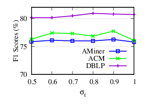
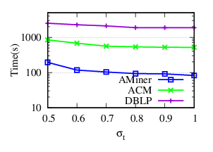
Exp-4.1: Impacts of σt. To evaluate the impacts of word-word similarity, we vary σt from 0.5 to 1, and fix other parameters to their default values. With σt increasing, fewer similar pairs of words are taken into consideration. σt = 1 means that we dismiss the word-word similarity. The accuracy and running time results of NDCC w.r.t. σt in AMiner, ACM and DBLP are plotted in Fig. 7(a) and Fig. 7(b), respectively.
The results show that (a) including word-word similarity can increase the accuracy performance of NDCC. Specifically, it improves F1 scores up to (0.59%, 2.21%, 0.26%) on (AMiner, ACM, DBLP), respectively, (b) small σt, such as 0.5, which means words pairs with low similarities are also considered, may decrease the accuracy results, (c) NDCC achieves relatively high accuracy in a wide range of σt, (d) the running time decreases with increasing σt because larger σt reduces the number of non-zero elements of WTT.
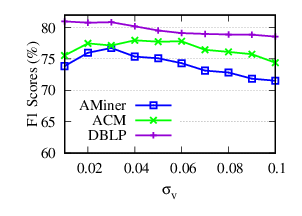
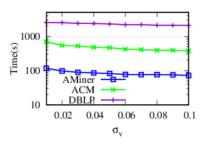
Exp-4.2: Impacts of σv. To evaluate the impacts of venue-venue similarity, we vary σv from 0.01 to 0.1 by step 0.01 and fix other parameters to their default values. Since most similarity scores of venue pairs are located in the range of (0, 0.1), we just range σv up to 0.1. The accuracy and running time results of NDCC w.r.t. different σv on AMiner, ACM and DBLP are plotted in Fig. 8(a) and Fig. 8(b), respectively.
The results tell us that (a) the usage of venue similarity can improve the accuracy performance significantly. Specifically, it improves the F1 scores up to (7.28%, 4.58%, 3.09%) on (AMiner, ACM, DBLP), respectively, (b) when σv is small, venue pairs with low similar scores are involved, which may decrease the accuracy results, (c) NDCC achieves relatively high F1 scores in a wide range of σv, (d) the running time goes down as σv increases, because higher threshold means that less similar venue pairs are considered.
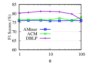
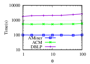
Exp-4.3: Impacts of θ. To evaluate the impacts of θ, we vary θ from 1 to 100 (1, 2, 5, 10, 20, 50, 100) and fix other parameters to their default values. The accuracy results and running time of NDCC w.r.t. θ on three datasets are plotted in Fig. 9.
The results show that (a) NDCC is robust to θ, (b) when θ is very large, for example, 100, (author, 2-hop coauthor) and (author, 2-hop coauthor name) relationships are used in similarity calculation for high ambiguous names, which impairs the accuracy performance. At the same time, it leads to more running time.
Summary. From these tests, we find the followings.
(1) Our approach NDCC is effective for scholar name disambiguation. Macro-F1 scores of NDCC are consistently higher than the compared methods in all datasets.
(2) Our approach NDCC is also very efficient. With speeding up strategies, NDCC could finish on DBLP, which contains over 3 million papers, within an hour.
(3) The author numbers detected by NDCC are reasonable.
(4) We provide insights of NDCC by experimentally demonstrating the effectiveness of its each step.
(5) Strategies dealing with sparsity improve the accuracy performance. Besides, NDCC introduces thresholds to word-word similarity, venue-venue similarity and author similarity measurement for the sake of practicability and flexibility of real-life applications. We have experimentally shown that NDCC is robust to these parameters.
In general, existing work for scholar name disambiguation can be divided into two classes: supervised [4], [14], [16], [17], [33], [36], [38], [42] and unsupervised [7], [9], [10], [18], [26], [27], [30], [32], [35], [37], [39], [40]. Supervised methods use labeled data to train a classifier, e.g., SVM [36] and random forests [16], [17], [33], which is then used to assign publications to different author entities. However, labeling data is time-consuming and impractical when the bibliography data is large. Unsupervised methods use clustering, e.g., agglomerative clustering [9], [18], [37], affinity propagation [10] and Markov clustering [39], or topic modeling [26], [27] to divide the set of author references into different subsets. Our work belongs to the second category.
There are three kinds of evidences that are commonly explored by disambiguation methods [11]: citation information [7], [36], web information [18], affiliation [5], and implicit evidence [26], [27]. Citation information is extracted directly from citation records, including author names, title, venue, publication year. Our work only uses citation information, and applies to most digital libraries. It is also known that the usage of new evidence, e.g., wiki [18], abstracts [30], [35], and homepages [35], usually improves the disambiguation performance. These methods are orthogonal to our method and can be combined to further improve the performance of our method.
Most existing name disambiguation methods are designed to tackle single name ambiguity and dismiss their connections. While in this study, we focus on scholar name disambiguation in a collective way. There are also some collective entity resolution methods that can be used to solve multiple name disambiguation problem [7], [13], [25]. However, they are not designed for scholar name disambiguation, as they mainly aim to deal with duplication problems in relational databases caused by different forms of the same names. Most of them need another clean knowledge base (KB) [13], [25], which is unavailable in most cases. [7] is a collective entity resolution method without a KB. However, it needs to store all pairs of similar author references and their similarity scores in a single queue. Its high space complexity keeps it away from large-scale data analytics.
Considering the connections of scholar names, we have proposed a collective approach to scholar name disambiguation. We have developed a novel metric to determine the author similarity by assembling the similarities of four features (coauthors, venues, titles and coauthor names). To deal with the sparsity problem, we have also introduced word-word and venue-venue similarities. As is shown in the experimental study, NDCC is both effective and efficient for scholar name disambiguation.
Our collective clustering method may have the potential for a more general setting, where multiple clustering problems need to be solved jointly, such as community detection in multiple networks [21], [22]. A couple of topics need further investigation. First, we are to combine new evidence to further improve the performance of our method. Second, we are to study NDCC in a dynamic scenario.
Acknowledgments
This work is supported in part by National Key R&D Program of China 2018AAA0102301, and NSFC 61925203 & U1636210, and Shenzhen Institute of Computing Sciences.
[1] DBLP, 2020. http://dblp.uni-trier.de/.
[2] Google Scholar, 2020. https://scholar.google.com/.
[3] Microsoft academic search, 2020. https://labs.cognitive. microsoft.com/en-us/project-academic-knowledge.
[4] M. A. Abdulhayoglu and B. Thijs. Use of researchgate and google cse for author name disambiguation. Scientometrics, 111(3):1965–1985, 2017.
[5] T. Backes. Effective unsupervised author disambiguation with relative frequencies. In JCDL, 2018.
[6] A. Barrena, A. Soroa, and E. Agirre. Alleviating poor context with background knowledge for named entity disambiguation. In ACL, 2016.
[7] I. Bhattacharya and L. Getoor. Collective entity resolution in relational data. TKDD, 1(1):5, 2007.
[8] S. Bird, E. Klein, and E. Loper. Natural language processing with Python: analyzing text with the natural language toolkit. ” O’Reilly Media, Inc.”, 2009.
[9] L. Cen, E. C. Dragut, L. Si, and M. Ouzzani. Author disambiguation by hierarchical agglomerative clustering with adaptive stopping criterion. In SIGIR, 2013.
[10] X. Fan, J. Wang, X. Pu, L. Zhou, and B. Lv. On graph-based name disambiguation. JDIQ, 2(2):10:1–10:23, 2011.
[11] A. A. Ferreira, M. A. Gonçalves, and A. H. Laender. A brief survey of automatic methods for author name disambiguation. SIGMOD Rec., 41(2):15–26, 2012.
[12] A. Glaser and J. Kuhn. Named entity disambiguation for little known referents: a topic-based approach. In COLING, 2016.
[13] A. Globerson, N. Lazic, S. Chakrabarti, A. Subramanya, M. Ringaard, and F. Pereira. Collective entity resolution with multi-focal attention. In ACL, 2016.
[14] D. Han, S. Liu, Y. Hu, B. Wang, and Y. Sun. Elm-based name disambiguation in bibliography. WWW, 18(2):253–263, 2015.
[15] J. Han, J. Pei, and M. Kamber. Data mining: concepts and techniques. Elsevier, 2011.
[16] M. Khabsa, P. Treeratpituk, and C. L. Giles. Large scale author name disambiguation in digital libraries. In IEEE BigData, 2014.
[17] M. Khabsa, P. Treeratpituk, and C. L. Giles. Online person name disambiguation with constraints. In JCDL, 2015.
[18] S. Li, G. Cong, and C. Miao. Author name disambiguation using a new categorical distribution similarity. In ECML/PKDD, 2012.
[19] X. Li, Y. Wu, M. Ester, B. Kao, X. Wang, and Y. Zheng. Semi-supervised clustering in attributed heterogeneous information networks. In WWW, 2017.
[20] J. Liu, S. Ma, R. Hu, C. Hu, and J. Huai. Athena: A ranking enabled scholarly search system. In WSDM, 2020.
[21] R. Liu, W. Cheng, H. Tong, W. Wang, and X. Zhang. Robust multi-network clustering via joint cross-domain cluster alignment. In ICDM, 2015.
[22] D. Luo, J. Ni, S. Wang, Y. Bian, X. Yu, and X. Zhang. Deep multi-graph clustering via attentive cross-graph association. In WSDM, 2020.
[23] S. Ma, C. Gong, R. Hu, D. Luo, C. Hu, and J. Huai. Query independent scholarly article ranking. In ICDE, 2018.
[24] T. Mikolov, K. Chen, G. Corrado, and J. Dean. Efficient estimation of word representations in vector space. In ICLR, 2013.
[25] W. Shen, J. Han, and J. Wang. A probabilistic model for linking named entities in web text with heterogeneous information networks. In SIGMOD, 2014.
[26] L. Shu, B. Long, and W. Meng. A latent topic model for complete entity resolution. In ICDE, 2009.
[27] Y. Song, J. Huang, I. G. Councill, J. Li, and C. L. Giles. Efficient topic-based unsupervised name disambiguation. In JCDL, 2007.
[28] Y. Sun and J. Han. Mining Heterogeneous Information Networks: Principles and Methodologies. Synthesis Lectures on Data Mining and Knowledge Discovery. Morgan & Claypool Publishers, 2012.
[29] M. J. Swain and D. H. Ballard. Color indexing. IJCV, 7(1):11–32, 1991.
[30] J. Tang, A. C. Fong, B. Wang, and J. Zhang. A unified probabilistic framework for name disambiguation in digital library. TKDE, 24(6):975–987, 2011.
[31] J. Tang, J. Zhang, L. Yao, J. Li, L. Zhang, and Z. Su. Arnetminer: extraction and mining of academic social networks. In SIGKDD, 2008.
[32] J. Tang, J. Zhang, D. Zhang, and J. Li. A unified framework for name disambiguation. In WWW, 2008.
[33] P. Treeratpituk and C. L. Giles. Disambiguating authors in academic publications using random forests. In JCDL, 2009.
[34] F. Wang, W. Wu, Z. Li, and M. Zhou. Named entity disambiguation for questions in community question answering. Knowledge-Based Systems, 126:68–77, 2017.
[35] X. Wang, J. Tang, H. Cheng, and S. Y. Philip. Adana: Active name disambiguation. In ICDM, 2011.
[36] X. Yin, J. Han, and S. Y. Philip. Object distinction: Distinguishing objects with identical names. In ICDE, 2007.
[37] B. Zhang and M. Al Hasan. Name disambiguation in anonymized graphs using network embedding. In CIKM, 2017.
[38] B. Zhang, M. Dundar, and M. Al Hasan. Bayesian non-exhaustive classification a case study: Online name disambiguation using temporal record streams. In CIKM, 2016.
[39] B. Zhang, T. K. Saha, and M. Al Hasan. Name disambiguation from link data in a collaboration graph. In ASONAM, 2014.
[40] S. Zhang, E. Xinhua, T. Huang, and F. Yang. Andmc: An algorithm for author name disambiguation based on molecular cross clustering. In DASFAA, 2019.
[41] Y. Zhang, Y. Xiong, X. Kong, S. Li, J. Mi, and Y. Zhu. Deep collective classification in heterogeneous information networks. In WWW, 2018.
[42] Y. Zhang, F. Zhang, P. Yao, and J. Tang. Name disambiguation in aminer: Clustering, maintenance, and human in the loop. In SIGKDD, 2018.