Random Walk on Multiple Networks
Dongsheng Luo, Yuchen Bian, Yaowei Yan, Xiong Yu, Jun Huan, Xiao Liu, Xiang Zhang
Abstract
Random Walk is a basic algorithm to explore the structure of networks, which can be used in many tasks, such as
local community detection and network embedding. Existing random walk methods are based on single networks that
contain limited information. In contrast, real data often contain entities with different types or/and from different sources,
which are comprehensive and can be better modeled by multiple networks. To take the advantage of rich information in
multiple networks and make better inferences on entities, in this study, we propose random walk on multiple networks, RWM.
RWM is flexible and supports both multiplex networks and general multiple networks, which may form many-to-many node
mappings between networks. RWM sends a random walker on each network to obtain the local proximity (i.e., node visiting
probabilities) w.r.t. the starting nodes. Walkers with similar visiting probabilities reinforce each other. We theoretically analyze
the convergence properties of RWM. Two approximation methods with theoretical performance guarantees are proposed for
efficient computation. We apply RWM in link prediction, network embedding, and local community detection. Comprehensive
experiments conducted on both synthetic and real-world datasets demonstrate the effectiveness and efficiency of RWM.
Index Terms
Random Walk, Complex Network, Local Community Detection, Link Prediction, Network Embedding
∙ D. Luo is with the Florida International University, Miami, FL, 33199.
E-mail: dluo@fiu.edu.
∙ Y. Bian is with Amazon Search Science and AI, USA.
E-mail: yuchbian@amazon.com.
∙ Y. Yan is with Meta Platforms, Inc., USA.
E-mail: yanyaw@meta.com.
∙ X. Liu, and X. Zhang are with the Pennsylvania State University, State College, PA 16802.
E-mail: {xxl213, xzz89}@psu.edu.
∙ X. Yu is with Case Western Reserve University.
E-mail: xxy21@case.edu
∙ J. Huan is with AWS AI Labs; work done before joining AWS.
E-mail: lukehuan@amazon.com*
1 Introduction
Networks (graphs) are natural representations of relational data in the real world, with vertices modeling entities and edges
describing relationships among entities. With the rapid growth of information, a large volume of network data is generated, such as
social networks [25], author collaboration networks [39], document citation networks [34], and biological networks [41]. In many
emerging applications, different types of vertices and relationships are obtained from different sources, which can be better modeled
by multiple networks.
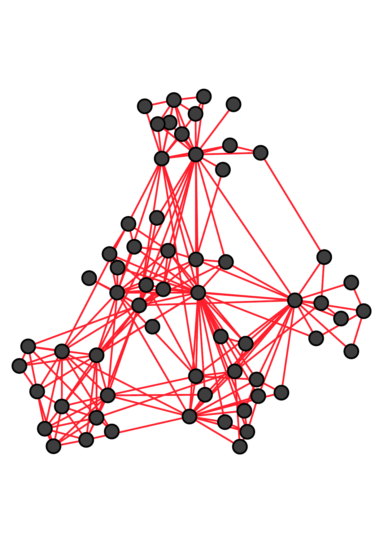
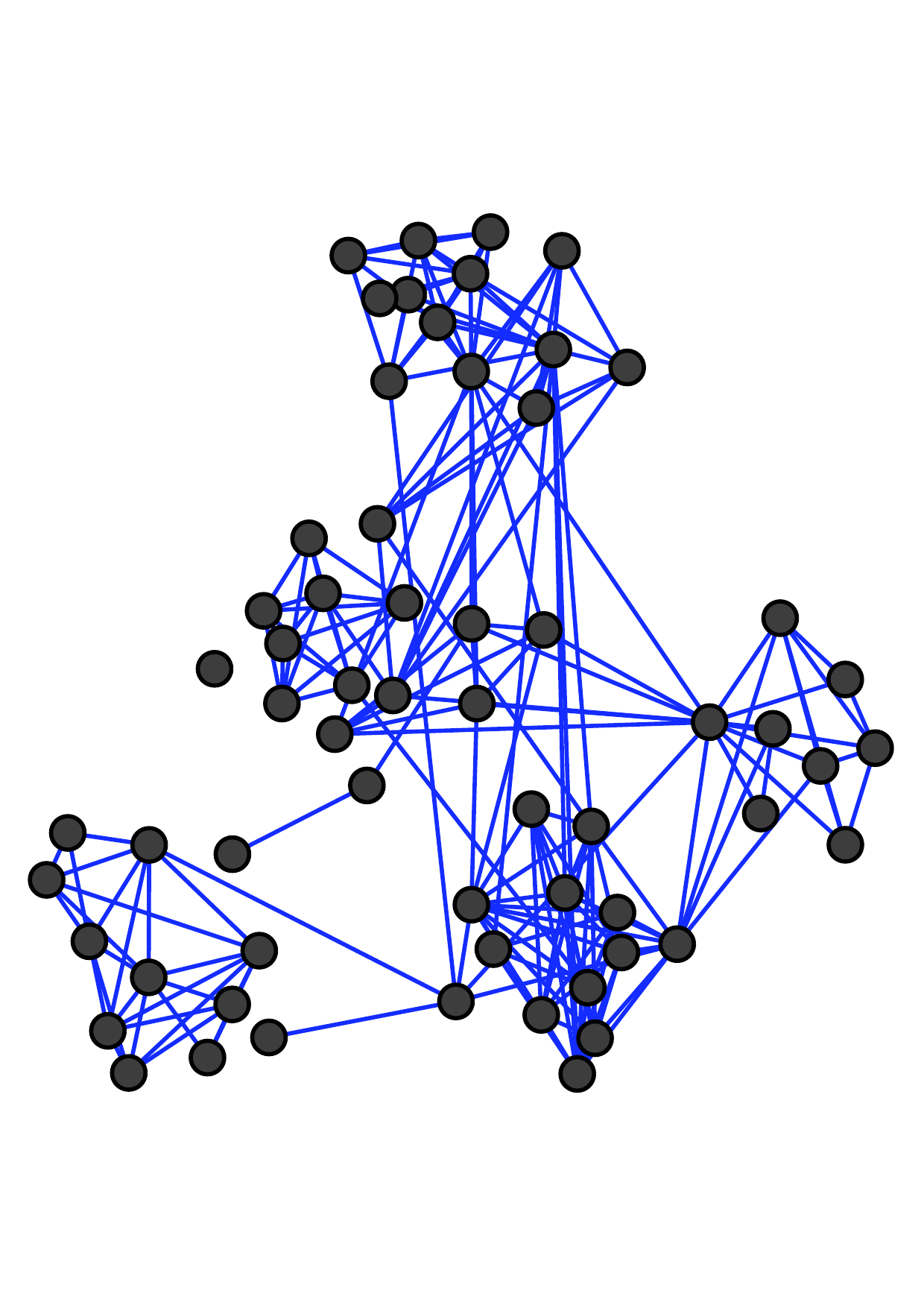
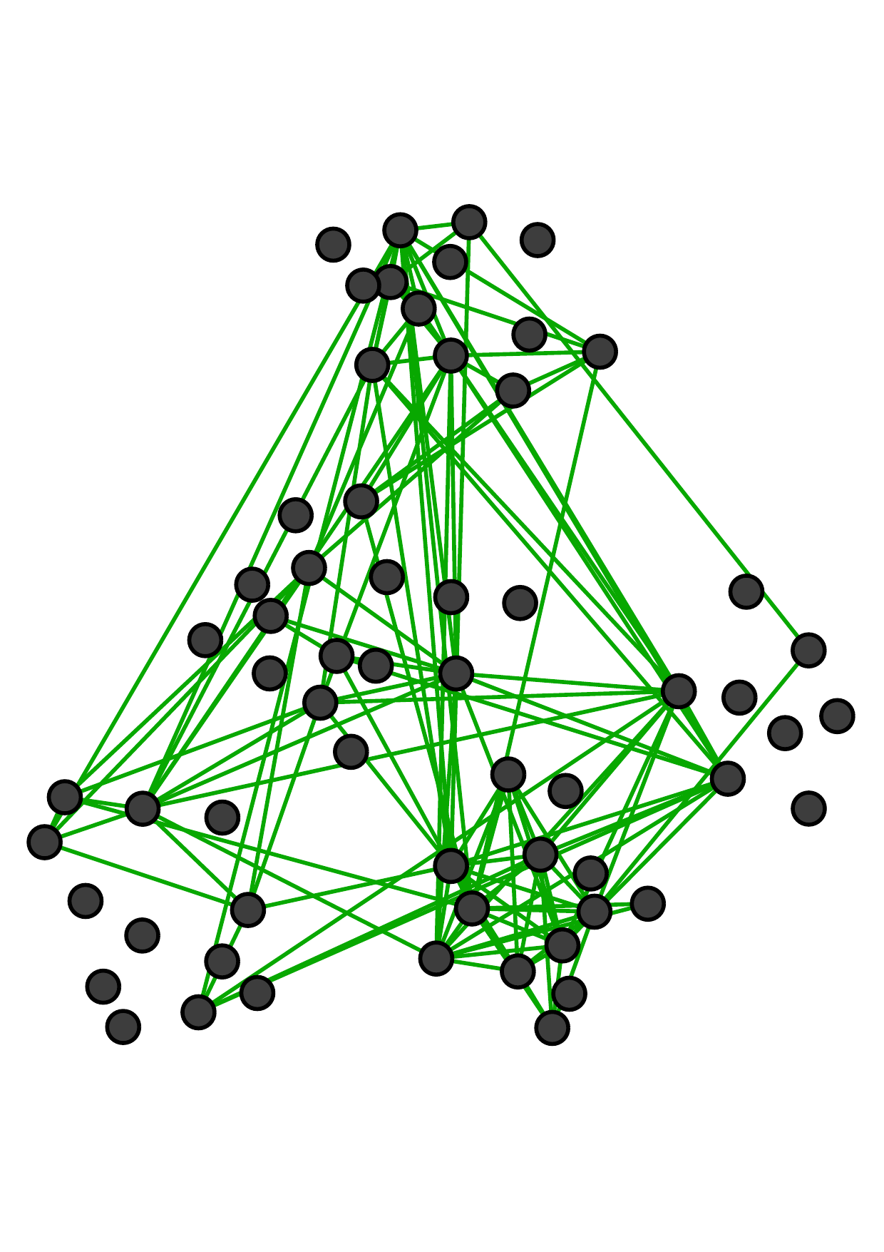
There are two main kinds of multiple networks. Fig. 1 shows an example of multiple networks with the same node set and
different types of edges (which are called multiplex networks [19, 37] or multi-layer networks). Each node represents an employee of a
university [18]. These three networks reflect different relationships between employees: co-workers, lunch-together, and
Facebook-friends. Notice that more similar connections exist between two offline networks (i.e., co-worker and lunch-together) than
that between offline and online relationships (i.e., Facebook-friends).
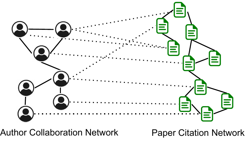
Fig. 2 is another example from the DBLP dataset with multiple domains of nodes and edges (which is called multi-domain
networks [40, 33]). The left part is the author-collaboration network and the right part is the paper-citation network. A cross-edge
connecting an author and a paper indicates that the author writes the paper. We see that authors and papers in the same research
field may have dense cross-links. Multiplex networks are a special case of multi-domain networks with the same set of nodes and
the cross-network relations are one-to-one mappings.
Given a starting node in a graph, we randomly move to one of its neighbors; then we move to a neighbor of the
current node at random etc,. This process is called random walk on the graph [30]. Random walk is an effective and
widely used method to explore the local structures in networks, which serves as the basis of many advanced tasks
such as network embedding [9, 15, 46, 47], link prediction [35], node/graph classification [21, 20], and graph
generation [8]. Various extensions, such as the random walk with restart (RWR) [49], second-order random walk [55], and
multi-walker chain [5] have been proposed to analyze the network structure. Despite the encouraging progress,
most existing random walk methods focus on a single network merely. Some methods merge the multiple networks
as a single network by summation and then apply traditional random walk[12]. However, these methods neglect
types of edges and nodes and assume that all layers have the same effect, which may be too restrictive in most
scenarios.
To this end, in this study, we propose a novel random walk method, RWM (Random Walk on Multiple networks), to explore
local structures in multiple networks. The key idea is to integrate complementary influences from multiple networks. We
send out a random walker on each network to explore the network topology based on corresponding transition
probabilities. For networks containing the starting node, the probability vectors of walkers are initiated with the starting
node. For other networks, probability vectors are initialized by transiting visiting probability via cross-connections
among networks. Then probability vectors of the walkers are updated step by step. The vectors represent walkers’
visiting histories. Intuitively, if two walkers share similar or relevant visiting histories (measured by cosine similarity
and transited with cross-connections), it indicates that the visited local typologies in corresponding networks are
relevant. And these two walkers should reinforce each other with highly weighted influences. On the other hand,
if visited local typologies of two walkers are less relevant, smaller weights should be assigned. We update each
walker’s visiting probability vector by aggregating other walkers’ influences at each step. In this way, the transition
probabilities of each network are modified dynamically. Compared to traditional random walk models where the transition
matrix is time-independent [2, 27, 22, 54, 53], RWM can restrict most visiting probability in the local subgraph
w.r.t. the starting node, in each network and ignore irrelevant or noisy parts. Theoretically, we provide rigorous
analyses of the convergence properties of the proposed model. Two speeding-up strategies are developed as well. We
conduct extensive experiments on real and synthetic datasets to demonstrate the advantages of our RWM model on
effectiveness and efficiency for local community detection, link prediction, and network embedding in multiple
networks.
Our contributions are summarized as follows.
-
We propose a novel random walk model, RWM, on multiple networks, which serves as a basic tool to analyze
multiple networks.
-
Fast estimation strategies and sound theoretical foundations are provided to guarantee the effectiveness and
efficiency of RWM.
-
Results of comprehensive experiments on synthetic and real multiple networks verify the advances of RWM.
2 Related Work
Random Walk. In the single network random walk, a random walker explores the network according to the node-to-node transition
probabilities, which are determined by the network topology. There is a stationary probability for visiting each node if the network
is irreducible and aperiodic [24]. Random walk is the basic tool to measure the proximity of nodes in the network. Based on the
random walk, various proximity measurement algorithms have been developed, among which PageRank [44], RWR [49],
SimRank [17], and MWC [5] have gained significant popularity. In PageRank, instead of merely following the transition probability,
the walker has a constant probability to jump to any node in the network at each time point. Random walk with restart, a.k.a.
personalized PageRank, is the query biased version of PageRank. At each time point, the walker has a constant probability to
jump back to the query (starting) node. SimRank aims to measure the similarity between two nodes based on the
principle that two nodes are similar if their neighbors are similar. With one walker starting from each node, the
SimRank value between two nodes represents the expected number of steps required before two walkers meet at the
same node if they walk in lock-step. MWC sends out a group of walkers to explore the network. Each walker is
pulled back by other walkers when deciding the next steps, which helps the walkers to stay as a group within the
cluster.
Very limited work has been done on the multiple network random walk. In [38], the authors proposed a classical random walk
with uniform categorical coupling for multiplex networks. They assign a homogeneous weight ω for all cross-network edges
connecting the same nodes in different networks. In [12], the authors propose a random walk method, where for each step the
walker has (1 - r) probability to stay in the same network and r probability to follow cross-network edges. However, both of
them are designed for multiplex networks and cannot be applied to general multiple networks directly. Further,
both ω and r are set manually and stay the same for all nodes, which means these two methods only consider the
global relationship between networks, which limits their applications in general and complex networks. In [58], the
authors propose a random walk method on multi-domain networks by including a transition matrix between different
networks. However, the transition matrix between networks is set manually and is independent of the starting
node(s).
Multiple Network Analysis. Recently, multiple networks have drawn increasing attention in the literature due to their capability in
describing graph-structure data from different domains [26, 40, 43, 14, 61, 59, 60, 56]. Under the multiple network setting, a wide
range of graph mining tasks have been extended to support more realistic real-life applications, including node
representation learning [40, 26, 14, 60], node clustering [11, 29, 43, 33], and link prediction [61, 59]. For example,
Multiplex Graph Neural Network is proposed to tackle the multi-behavior recommendation problem [61]. In [59], the
authors consider the relational heterogeneity within multiplex networks and propose a multiplex heterogeneous graph
convolutional network (MHGCN) to learn node representations in heterogeneous networks. Compared to previous ones,
MHGCN can adaptively extract useful meta-path interactions. Instead of focusing on a specific graph mining task, in
this paper, we focus on designing a novel random walk model that can be used in various tasks as a fundamental
component.
3 Random Walk on Multiple Networks
In this section, we first introduce notations. Then the reinforced updating mechanism among random walkers in RWM is
proposed.
Table 1
Main notations
|
|
| Notation | Definition |
|
|
| K | The number of networks |
| Gi | The ith network. |
| V i | The node set of Gi |
| Ei | The edge set of Gi |
| Pi | Column-normalized transition matrix of Gi. |
| Ei-j | The cross-edge set between network Gi and Gj |
| Si→j | Column-norm. cross-trans. mat. from V i to V j |
| uq | A given starting node uq from V q |
| eq | One-hot vector with only one value-1 entry for uq |
| xi(t) | Node visit. prob. vec. of the ith walker in G
i at t |
| W(t) | Relevance weight matrix at time t |
 i(t) i(t) | Modified trans. mat. for the ith walker in G
i at t |
| α,λ,θ | restart factor, decay factor, covering factor. |
| |
3.1 Notations
Suppose that there are K undirected networks, the ith (1 ≤ i ≤ K) network is represented by Gi = (V i,Ei)
with node set V i and edge set Ei. We denote its transition matrix as a column-normalized matrix Pi ∈ℝ|V i|×|V i|.
The (v,u)th entry Pi(v,u) represents the transition probability from node u to node v in V i. Then the uth column
Pi(:,u) is the transition distribution from node u to all nodes in V i. Next, we denote Ei-j the cross-connections
between nodes in two networks V i and V j. The corresponding cross-transition matrix is Si→j ∈ℝ|V j|×|V i|. Then the
uth column Si→j(:,u) is the transition distribution from node u ∈ V i to all nodes in V j. Note that Si→j≠Sj→i.
And for the multiplex networks with the same node set (e.g., Fig. 1), Si→j is just an identity matrix I for arbitrary
i,j.
Suppose we send a random walker on Gi, we let xi(t) be the node visiting probability vector in Gi at time t. Then the updated
vector xi(t+1) = Pixi(t) means the probability transiting among nodes in Gi. And Si→jxi(t) is the probability vector propagated
into Gj from Gi. Important notations are summarized in Table 1.
3.2 Reinforced Updating Mechanism
In RWM, we send out one random walker for each network. Initially, for the starting node uq ∈ Gq, the corresponding walker’s xq(0) = eq
where eq is a one-hot vector with only one value-1 entry corresponding to uq. For other networks Gi(i≠q), we initialize xi(0) by xi(0) = Sq→ixq(0).
That is :
To update ith walker’s vector xi(t), the walker not only follows the transition probabilities in the corresponding network Gi, but
also obtains influences from other networks. Intuitively, networks sharing relevant visited local structures should influence each
other with higher weights. And the ones with less relevant visited local structures have fewer effects. We measure the relevance of
visited local structures of two walkers in Gi and Gj with the cosine similarity of their vectors xi(t) and xj(t). Since different
networks consist of different node sets, we define the relevance as cos(xi(t),Sj→ixj(t)). Notice that when t increases, walkers will
explore nodes further away from the starting node. Thus, we add a decay factor λ (0 < λ < 1) in the relevance to emphasize the
similarity between local structures of two different networks within a shorter visiting range. In addition, λ can
guarantee and control the convergence of the RWM model. Formally, we let W(t) ∈ℝK×K be the local relevance
matrix among networks at time t and we initialize it with identity matrix I. We update each entry W(t)(i,j) as
follow:
For the ith walker, influences from other networks are reflected in the dynamic modification of the original transition matrix Pi
based on the relevance weights. Specifically, the modified transition matrix of Gi is:
where Sj→iPjSi→j represents the propagation flow pattern Gi → Gj → Gi (counting from the right side) and
 (t)(i,j) =
  is the row-normalized local relevance weights from Gj to Gi. To guarantee the stochastic property of the
transition matrix, we also column-normalize
is the row-normalized local relevance weights from Gj to Gi. To guarantee the stochastic property of the
transition matrix, we also column-normalize  i(t) after each update.
At time t + 1, the visiting probability vector of the walker on Gi is updated:
Different from the classic random walk model, transition matrices in RWM dynamically evolve with local relevance influences
among walkers from multiple networks. As a result, the time-dependent property enhances RWM with the power of aggregating
relevant and useful local structures among networks.
Next, we theoretically analyze the convergence properties. First, in Theorem 1, we present the weak convergence property [5] of
the modified transition matrix i(t). The convergence of the visiting probability vector will be provided in Theorem
3.
For the multiple networks with the same node set (i.e., multiplex networks), we have a faster convergence rate.
Proof. In the multiplex networks, cross-transition matrices are just I, so the stochastic property of i(t) can be naturally
guaranteed without the column-normalization of i(t). We then define Δ(t + 1) =∥i(t+1) -i(t) ∥∞.
Based on Eq. (3) and Eq. (2), we have
where Li = {j| (t+1)(i,j) >=
  (t)(i,j)}, and Li = {1,2...,K}- Li. Since all entries in Pj are non-negative,
for all j, all entries in the first part are non-negative and all entries in the second part is non-positive. Thus, we
have
(t)(i,j)}, and Li = {1,2...,K}- Li. Since all entries in Pj are non-negative,
for all j, all entries in the first part are non-negative and all entries in the second part is non-positive. Thus, we
have
Since for all i, score vector xi(t) is non-negative, we have cos(xi(t),xk(t)) ≥ 0. Thus, ∑
kW(t+1)(i,k) ≥∑
kW(t)(i,k). For the
first part, we have
Similarly, we can prove the second part has the same bound.
Thus, we have
Then, we know Δ(t + 1) ≤ ϵ when t > ⌈log λ ⌉.
⌉.
Next, we consider the general case. In Theorem 1, we discuss the weak convergence of the modified transition
matrix i(t) in general multiple networks. Because after each iteration, i(t) needs to be column-normalized to
keep the stochastic property, we let  i(t) represent the column-normalized one. Then Theorem 1 is for the residual
Δ(t + 1) =∥
i(t) represent the column-normalized one. Then Theorem 1 is for the residual
Δ(t + 1) =∥ i(t+1) -
 i(t) ∥∞.
Based on Eq. (2), we have for all t,  ≤∑
zi(t)(z,y) ≤ 1.
≤∑
zi(t)(z,y) ≤ 1.
We denote min{i(t+1)(x,y),i(t)(x,y)} as p and min{∑
zi(t+1)(z,y),∑
zi(t)(z,y)} as m. From the proof of Theorem 2 ,
we know that
and
Then, we have
When t > ⌈-log λ(K2|V i|)⌉, we have λtK2|V i|≤ 1. Thus,
Then, it’s derived that Δ(t + 1) ≤ ϵ when t > ⌈log λ ⌉. __
⌉. __
3.3 RWM With Restart Strategy
RWM is a general random walk model for multiple networks and can be further customized into different variations. In this
section, we integrate the idea of random walk with restart (RWR) [49] into RWM.
In RWR, at each time point, the random walker explores the network based on topological transitions with α(0 < α < 1)
probability and jumps back to the starting node with probability 1 -α. The restart strategy enables RWR to obtain proximities of all
nodes to the starting node.
Similarly, we apply the restart strategy for RWM in updating visiting probability vectors. For the ith walker, we
have:
where i(t) is obtained by Eq. (3). Since the restart component does not provide any information for the visited local
structure, we dismiss this part when calculating local relevance weights. Therefore, we modify the cos(⋅,⋅) in Eq. (2) and
have:
Theorem 3. Adding the restart strategy in RWM does not affect the convergence properties in Theorems 1 and 2. The visiting vector
xi(t)(1 ≤ i ≤ K) will also converge.
We skip the proof here. The main idea is that λ first guarantees the weak convergence of i(t) (λ has the same effect as in
Theorem 1). After obtaining a converged i(t), Perron-Frobenius theorem [31] can guarantee the convergence of xi(t) with a similar
convergence proof of the traditional RWR model.
3.4 Time complexity of RWM.
As a basic method, we can iteratively update vectors until convergence or stop the updating at a given number of iterations T .
Algorithm 1 shows the overall process.
In each iteration, for the ith walkers (line 4-5), we update xi(t+1) based on Eq. (3) and (5) (line 4). Note that we do not compute
the modified transition matrix i(t) and output. If we substitute Eq. (3) in Eq. (5), we have a probability propagation
Sj→iPjSi→jxi(t) which reflects the information flow Gi → Gj → Gi. In practice, a network is stored as an adjacent list. So we only
need to update the visiting probabilities of direct neighbors of visited nodes and compute the propagation from right
to left. Then calculating Sj→iPjSi→jxi(t) costs O(|V i| + |Ei-j| + |Ej|). And the restart addition in Eq. (5) costs
O(|V i|). As a result, line 4 costs O(|V i| + |Ei| + ∑
j≠i(|Ei-j| + |Ej|)) where O(|Ei|) is from the propagation in Gi
itself.
In line 5, based on Eq. (6), it takes O(|Ei-j| + |V j|) to get Sj→ixj(t) and O(|V i|) to compute cosine similarities. Then
updating W(i,j) (line 5) costs O(|Ei-j| + |V i| + |V j|). In the end, normalization (line 6) costs O(K2) which can be
ignored.
In summary, with T iterations, power iteration method for RWM costs O((∑
i|V i| + ∑
i|Ei| + ∑
i≠j|Ei-j|)KT). For the
multiplex networks with the same node set V , the complexity shrinks to O((∑
i|Ei| + K|V |)KT) because of the one-to-one
mappings in Ei-j.
Note that power iteration methods may propagate probabilities to the entire network. Next, we present two speeding-up
strategies to restrict the probability propagation into only a small subgraph around the starting node.
___________________________________________________________________________________________________
Algorithm 1: Random walk on multiple networks____________________________________________________________________________________________________________________________
Input: Transition matrices {Pi}i=1K, cross-transition matrices {S
i→j}i≠j, tolerance ϵ, starting node uq ∈Gq, decay factor λ, restart
factor α, iteration number T
Output: Visiting prob. vec. for K walkers ({xi(T)}
i=1K)
1Initialize {xi(0)}
i=1K based on Eq. (1), and W(0) =  (0) = I;
2for t ←0 to T do
3
4
5for i ←1 to K do
6
7
8calculate xi(t+1) according to Eq. (3) and (5);
9calculate W(t+1) according to Eq. (6);
10
(0) = I;
2for t ←0 to T do
3
4
5for i ←1 to K do
6
7
8calculate xi(t+1) according to Eq. (3) and (5);
9calculate W(t+1) according to Eq. (6);
10 (t+1) ← row-normalize W(t+1);
____________________________________________________________________________________________________________________________________________________________
4 Speeding Up
In this section, we introduce two approximation methods that not only dramatically improve computational efficiency but also
guarantee performance.
4.1 Early Stopping
With the decay factor λ, the modified transition matrix of each network converges before the visiting score vector does. Thus, we
can approximate the transition matrix with early stopping by splitting the computation into two phases. In the first phase, we
update both transition matrices and score vectors, while in the second phase, we keep the transition matrices static and only update
score vectors.
Now we give the error bound between the early-stopping updated transition matrix and the power-iteration updated one. In Gi,
we denote i(∞) the converged modified transition matrix.
In Gi(1 ≤ i ≤ K), when properly selecting the split time Te, the following theorem demonstrates that we can securely
approximate the power-iteration updated matrix i(∞) with i(Te).
Proof. According to the proof of Theorem 1, when Te > ⌈-log λ(K2|V i|)⌉, we have
So we can select Te = ⌈log λ ⌉ such that when t > Te, ∥i(∞) -
i(t) ∥
∞ < ϵ. __
⌉ such that when t > Te, ∥i(∞) -
i(t) ∥
∞ < ϵ. __
The time complexity of the first phase is O((∑
i|V i| + ∑
i|Ei| + ∑
i≠j|Ei-j|)KTe).
___________________________________________________________________________________________________
Algorithm 2: Partial Updating______________________________________________________________________________________________________________________________________________________________
Input: xi(t), x
i(0), {P
i}i=1K, {S
i→j}i≠j, λ, α, θ
Output: approximation score vector  i(t+1)
1initialize an empty queue que;
2initialize a zero vector xi0(t) with the same size with x
i(t);
3que.push(Q) where Q is the node set with positive values in xi(0); mark nodes in Q as visited;
4cover ←0;
5while que is not empty and cover < θ do
6
7
8u ←que.pop();
9mark u as visited;
10for each neighbor node v of u do
11
12
13if v is not marked as visited then
14
15
16que.push(v);
17xi0(t)[u] ←x
i(t)[u];
18cover ←cover + xi(t)[u];
19Update
i(t+1)
1initialize an empty queue que;
2initialize a zero vector xi0(t) with the same size with x
i(t);
3que.push(Q) where Q is the node set with positive values in xi(0); mark nodes in Q as visited;
4cover ←0;
5while que is not empty and cover < θ do
6
7
8u ←que.pop();
9mark u as visited;
10for each neighbor node v of u do
11
12
13if v is not marked as visited then
14
15
16que.push(v);
17xi0(t)[u] ←x
i(t)[u];
18cover ←cover + xi(t)[u];
19Update  i(t+1) based on Eq. (7);
______________________________________________________________________________________________________________________________________________________________________
4.2 Partial Updating
In this section, we propose a heuristic strategy to further speed up the vector updating in Algorithm 1 (line 4) by only updating a
subset of nodes that covers most probabilities.
Specifically, given a covering factor θ ∈ (0,1], for walker i, in the tth iteration, we separate xi(t) into two non-negative vectors,
xi0(t) and Δxi(t), so that xi(t) = xi0(t) + Δxi(t), and ∥xi0(t) ∥1 ≥ θ. Then, we approximate xi(t+1) with
 i(t+1) = α
i(t)x
i0(t) + (1 - α ∥x
i0(t) ∥
1)xi(0) i(t+1) = α
i(t)x
i0(t) + (1 - α ∥x
i0(t) ∥
1)xi(0) | | (7) |
Thus, we replace the updating operation of xi(t+1) in Algorithm 1 (line 4) with  i(t+1). The details are shown in Algorithm 2.
Intuitively, nodes close to the starting node have higher scores than nodes far away. Thus, we utilize the breadth-first search (BFS) to
expand xi0(t) from the starting node set until ∥xi0(t) ∥1 ≥ θ (lines 3-12). Then, in line 13, we approximate the score vector in the
next iteration according to Eq. (7).
i(t+1). The details are shown in Algorithm 2.
Intuitively, nodes close to the starting node have higher scores than nodes far away. Thus, we utilize the breadth-first search (BFS) to
expand xi0(t) from the starting node set until ∥xi0(t) ∥1 ≥ θ (lines 3-12). Then, in line 13, we approximate the score vector in the
next iteration according to Eq. (7).
Let V i0(t) be the set of nodes with positive values in xi0(t), and |Ei0(t)| be the summation of out-degrees of nodes in V i0(t). Then
|Ei0(t)|≪|Ei| dramatically reduces the number of nodes to update in each iteration.
5 An Exemplar application of RWM
Random walk based methods are routinely used in various tasks, such as local community detection [2, 1, 27, 22, 6, 7, 4, 57, 51],
link prediction [35], and network embedding [9, 15, 46, 47]. In this section, we take the local community
detection as an example to show the application of the proposed RWM. As a fundamental task in large network
analysis, local community detection has attracted extensive attention recently. Unlike the time-consuming global
community detection, the goal of local community detection is to detect a set of nodes with dense connections (i.e.,
the target local community) that contains a given query node or a query node set. Specifically, given a query
node uq
in the query network Gq, the target of local community detection in multiple networks is to detect relevant local communities in all
networks Gi(1 ≤ i ≤ K).
To find the local community in network Gi, we follow the common process in the literature [2, 5, 22, 58]. By setting the query
node as the starting node, we first apply RWM with restart strategy to calculate the converged score vector xi(T), according to which
we sort nodes. T is the number of iterations. Suppose there are L non-zero elements in xi(T), for each l (1 ≤ l ≤ L), we compute the
conductance of the subgraph induced by the top l ranked nodes. The node set with the smallest conductance will be considered as
the detected local community.
6 Experiments
We perform comprehensive experimental studies to evaluate the effectiveness and efficiency of the
proposed methods. Our algorithms are implemented with C++. The code and data used in this work are
available.
All experiments are conducted on a PC with Intel Core I7-6700 CPU and 32 GB memory, running 64-bit Windows
10.
6.1 Datasets
Datasets. Eight real-world datasets are used to evaluate the effectiveness of the selected methods. Statistics are summarized in
Table 2.
∙ RM [18] has 10 networks, each with 91 nodes. Nodes represent phones and one edge exists if two phones detect each other under
a mobile network. Each network describes connections between phones in a month. Phones are divided into two communities
according to their owners’ affiliations.
∙ BrainNet [50] has 468 brain networks, one for each participant. In the brain network, nodes represent human
brain regions and an edge depicts the functional association between two regions. Different participants may have
different functional connections. Each network has 264 nodes, among which 177 nodes are studied to belong to 12
high-level functional systems, including auditory, memory retrieval, visual , etc. Each functional system is considered a
community.
The other four are general multiple networks with different types of nodes and edges and many-to-many cross-edges between
nodes in different networks.
∙ 6-NG & 9 -NG [40] are two multi-domain network datasets constructed from the 20-Newsgroup dataset. 6 -NG contains 5
networks of sizes {600, 750, 900, 1050, 1200} and 9 -NG consists of 5 networks of sizes {900, 1125, 1350, 1575, 1800}. Nodes
represent news documents and edges describe their semantic similarities. The cross-network relationships are measured by cosine
similarity between two documents from two networks. Nodes in the five networks in 6 -NG and 9 -NG are selected from 6 and 9
newsgroups, respectively. Each newsgroup is considered a community.
∙ Citeseer [28] is from an academic search engine, Citeseer. It contains a researcher collaboration network, a paper citation network,
and a paper similarity network. The collaboration network has 3,284 nodes (researchers) and 13,781 edges (collaborations). The
paper citation network has 2,035 nodes (papers) and 3,356 edges (paper citations). The paper similarity network has 10,214 nodes
(papers) and 39,411 edges (content similarity). There are three types of cross-edges: 2,634 collaboration-citation relations, 7,173
collaboration-similarity connections, and 2,021 citation-similarity edges. 10 communities of authors and papers are labeled based on
research areas.
∙ DBLP [48] consists of an author collaboration network and a paper citation network. The collaboration network has 1,209,164
nodes and 4,532,273 edges. The citation network consists of 2,150,157 papers connected by 4,191,677 citations. These two networks
are connected by 5,851,893 author-paper edges. From one venue, we form an author community by extracting the ones who
published more than 3 papers in that venue. We select communities with sizes ranging from 5 to 200, leading to 2,373
communities.
The above six datasets are with community information. We also include two datasets without label information for link
prediction tasks only.
∙ Athletics [42]: is a directed and weighted multiplex network dataset, obtained from Twitter during an exceptional event: the 2013
World Championships in Athletics. The multiplex network makes use of 3 networks, corresponding to retweets, mentions and
replies observed between 2013-08-05 11:25:46 and 2013-08-19 14:35:21. There are 88,804 nodes and (104,959, 92,370, 12,921) edges in
each network, respectively.
∙ Genetic [13] is a multiplex network describing different types of genetic interactions for organisms in the Biological General
Repository for Interaction Datasets (BioGRID, thebiogrid.org), a public database that archives and disseminates genetic and protein
interaction data from humans and model organisms. There are 7 networks in the multiplex network, including physical association,
suppressive genetic interaction defined by inequality, direct interaction, synthetic genetic interaction defined by inequality,
association, colocalization, and additive genetic interaction defined by inequality. There are 6,570 nodes and 282,754
edges.
Table 2
Statistics of datasets
|
|
|
|
|
| Dataset | #Net. | #Nodes | | |
|
|
|
|
|
| RM | 10 | 910 | 14,289 | – |
| BrainNet | 468 | 123,552 | 619,080 | – |
| Athletics | 3 | 88,804 | 210250 | - |
| Genetic | 7 | 6,570 | 28,2754 | - |
|
|
|
|
|
| 6 -NG | 5 | 4,500 | 9,000 | 20,984 |
| 9 -NG | 5 | 6,750 | 13,500 | 31,480 |
| Citeseer | 3 | 15,533 | 56,548 | 11,828 |
| DBLP | 2 | 3,359,321 | 8,723,940 | 5,851,893 |
| |
Table 3
Accuracy performances comparison
|
|
|
|
|
|
|
| Method | RM | BrainNet | 6 -NG | 9 -NG | Citeseer | DBLP |
|
|
|
|
|
|
|
| RWR | 0.621 | 0.314 | 0.282 | 0.261 | 0.426 | 0.120 |
| MWC | 0.588 | 0.366 | 0.309 | 0.246 | 0.367 | 0.116 |
| QDC | 0.150 | 0.262 | 0.174 | 0.147 | 0.132 | 0.103 |
| LEMON | 0.637 | 0.266 | 0.336 | 0.250 | 0.107 | 0.090 |
| k-core | 0.599 | 0.189 | 0.283 | 0.200 | 0.333 | 0.052 |
|
|
|
|
|
|
|
| MRWR | 0.671 | 0.308 | 0.470 | 0.238 | 0.398 | 0.126 |
| ML-LCD | 0.361 | 0.171 | - | - | - | - |
|
|
|
|
|
|
|
| RWM (ours) | 0.732* | 0.403* | 0.552* | 0.277* | 0.478* | 0.133* |
|
|
|
|
|
|
|
|
|
|
|
|
|
|
| Improve | 9.09% | 10.11% | 17.4% | 6.13% | 12.21% | 5.56% |
|
|
|
|
|
|
|
| *We do student-t test between RWM and the second best method MRWR
| (* corresponds to p < 0.05).
| |
6.2 Local community detection
6.2.1 Experimental setup
We compare RWM with seven state-of-the-art local community detection methods. RWR [49] uses a lazy variation of random
walk to rank nodes and sweeps the ranked nodes to detect local communities. MWC [5] uses the multi-walk chain model to
measure node proximity scores. QDC [54] finds local communities by extracting query biased densest connected subgraphs.
LEMON [27] is a local spectral approach. k-core [3] conducts graph core-decomposition and queries the community containing the
query node. Note that these five methods are for single networks. The following two are for multiple networks. ML-LCD [16]
uses a greedy strategy to find the local communities on multiplex networks with the same node set. MRWR [58]
only focuses on the query network. Besides, without prior knowledge, MRWR treats other networks contributing
equally.
For our method, RWM, we adopt two approximations and set ϵ = 0.01,θ = 0.9. Restart factor α and decay factor λ are searched
from 0.1 to 0.9. Extensive parameter studies are conducted in Sec. 6.2.3. For baseline methods, we tune parameters according to their
original papers and report the best results. Specifically, for RWR, MWC, and MRWR, we tune the Restart factor from 0.1 to 0.9. Other
parameters in MWC are kept the default values [5]. For QDC, we follow the instruction from the original paper
and search the decay factor from 0.6 to 0.95 [54]. For LEMON [27], the minimum community size and expand
step are set to 5 and 6, respectively. For ML-LCD, we adopt the vanilla Jaccard similarity as the node similarity
measure [16].
6.2.2 Effectiveness Evaluation
Evaluation on detected communities. For each dataset, in each experiment trial, we randomly pick one node with label information
from a network as the query. Our method RWM can detect all query-relevant communities from all networks, while all baseline
methods can only detect one local community in the network containing the query node. Thus, in this section, to be fair, we only
compare detected communities in the query network. In Sec. 6.2.4, we also verify that RWM can detect relevant and meaningful
local communities from other networks.
Each experiment is repeated 1000 trials, and the Macro-F1 scores are reported in Table 3. Note that ML-LCD can only be applied
to the multiplex network with the same node set.
From Table 3, we see that, in general, random walk based methods including RWR, MWC, MRWR, and RWM perform better
than others. It demonstrates the advance of applying random walk for local community detection. Generally, the size of
detected communities by QDC is very small, while that detected by ML-LCD is much larger than the ground truth.
k-core suffers from finding a proper node core structure with a reasonable size, it either considers a very small
number of nodes or the whole network as the detected result. Second, performances of methods for a single network,
including RWR, MWC, QDC, and LEMON, are relatively low, since the single networks are noisy and incomplete.
MRWR achieves the second best results on 6 -NG, RM, and DBLP but performs worse than RWR and MWC on
other datasets. Because not all networks provide equal and useful assistance for detection, treating all networks
equally in MRMR may introduce noises and decrease performance. Third, our method RWM achieves the highest
F1-scores on all datasets and outperforms the second best methods by 6.13% to 17.4%. We conduct student-t tests
between our method RWM and the second best method, MRWR. Low p-values (< 0.05) indicate that our results are
statistically significant. This is because RWM can actively aggregate information from highly relevant local structures
in other networks during updating visiting probabilities. We emphasize that only RWM can detect relevant local
communities from other networks except for the network containing the query node. Please refer to Sec. 6.2.4 for
details.
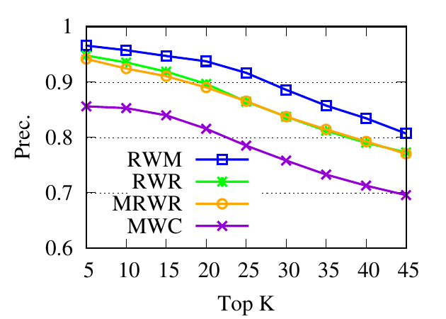
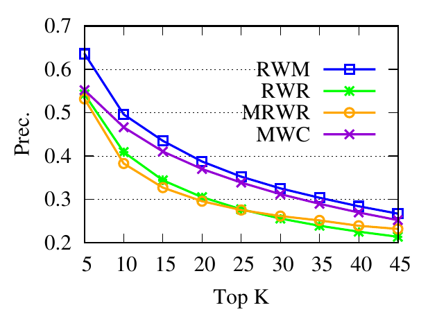
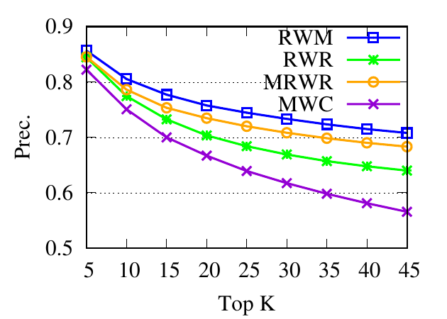
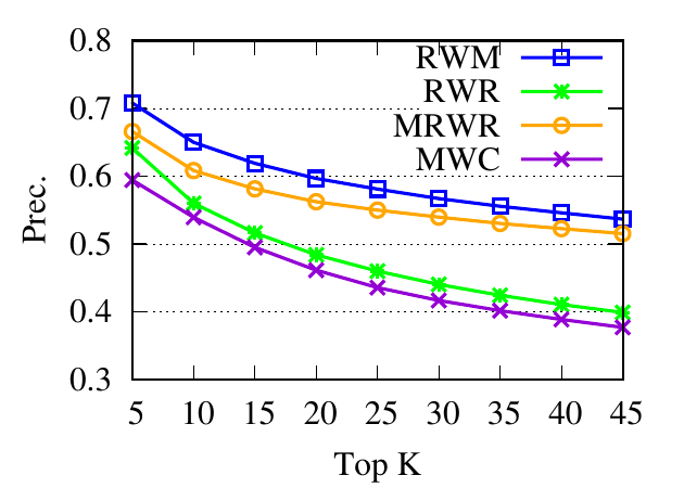
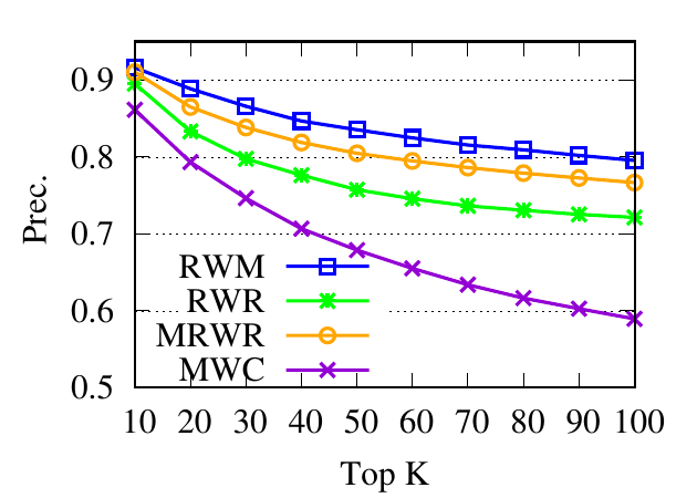
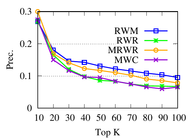
Ranking evaluation. To gain further insight into why RWM outperforms others, we compare RWM with other random walk based
methods, i.e., RWR, MWC, and MRWR, as follows. Intuitively, nodes in the target local community should be assigned with high
proximity scores w.r.t. the query node. Then we check the precision of top-ranked nodes based on score vectors of those models, i.e.,
prec. = (|top-knodes ∩ ground truth|)∕k
The precision results are shown in Fig. 3. First, we can see that the precision scores of the selected methods decrease when the
size of the detected community k increases. Second, our method consistently outperforms other random walk-based methods.
Results indicate that RWM ranks nodes in the ground truth more accurately. Since ranking is the basis of a random walk based
method for local community detection, better node-ranking generated by RWM leads to high-quality communities (Table
3).
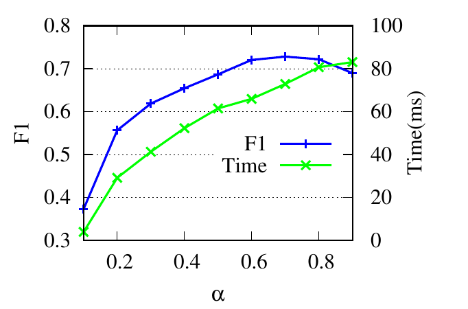
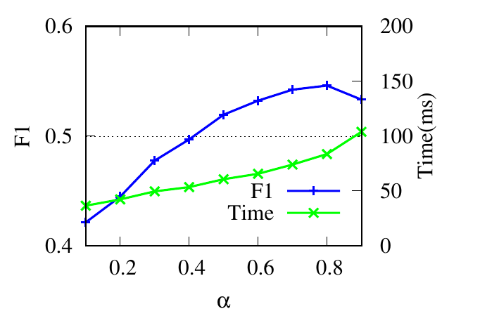
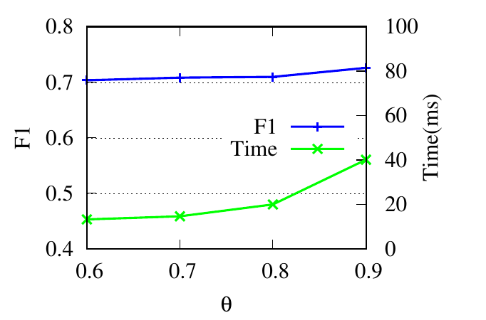
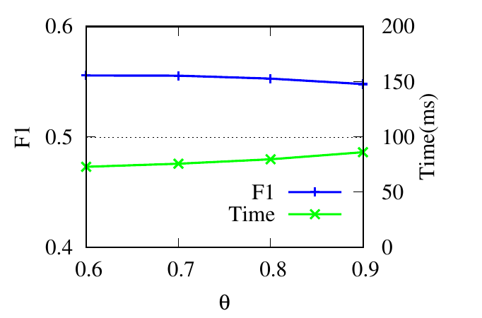
6.2.3 Parameter Study
In this section, we show the effects of the four important parameters in RWM: the restart factor α, the decay factor λ, tolerance
ϵ for early stopping, and the covering factor θ in the partial updating. We report the F1 scores and running time
on two representative datasets RM and 6 -NG. Note that ϵ and θ control the trade-off between running time and
accuracy.
The parameter α controls the restart of a random walker in Eq. (5). The F1 scores and the running time w.r.t. α are shown in
Fig. 4(a) and Fig. 4(b). When α is small, the accuracy increases as α increases because larger α encourages further exploration.
When α reaches an optimal value, the accuracy begins to drop slightly. Because a large α impairs the locality property of the restart
strategy. The running time increases when α increases because larger α requires more iterations for score vectors to
converge.
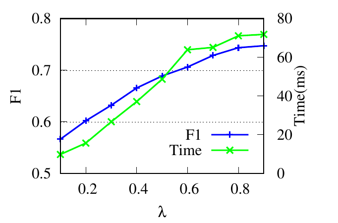
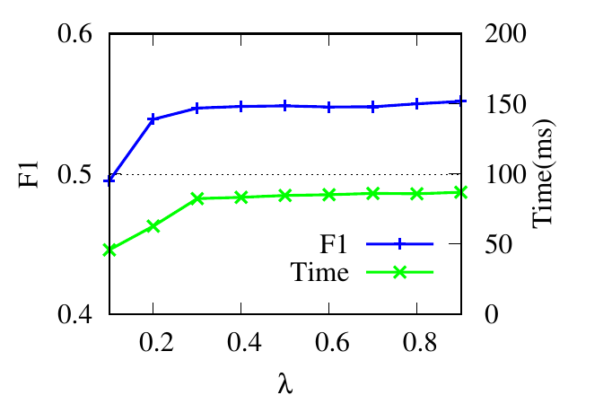
λ controls the updating of the relevance weights in Eq. (6). Results in Fig. 4(c) and Fig. 4(d) reflect that for RM, RWM
achieves the best result when λ = 0.9. This is because large λ ensures that enough neighbors are included when
calculating relevance similarities. For 6 -NG, RWM achieves high accuracy in a wide range of λ. For the running time,
according to Theorem 4, larger λ results in larger Te, i.e., more iterations in the first phase, and longer running
time.
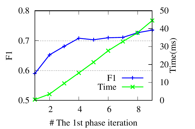
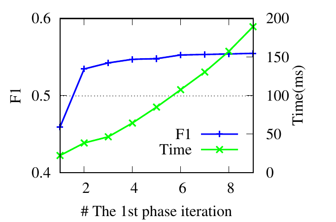
ϵ controls Te, the splitting time in the first phase. Instead of adjusting ϵ, we directly tune Te. Theoretically, a larger Te (i.e., a
smaller ϵ) leads to more accurate results. Based on results shown in Fig. 4(e) and Fig. 4(f), we notice that RWM achieves good
performance even with a small Te in the first phase. The running time decreases significantly as well. This demonstrates the
rationality of early stopping.
θ controls the number of updated nodes (in Sec. 4.2). In Fig. 4(g) and 4(h), we see that the running time decreases along with θ
decreasing because a smaller number of nodes are updated. The consistent accuracy performance shows the effectiveness of the
speeding-up strategy.
6.2.4 Case Studies
BrainNet and DBLP are two representative datasets for multiplex networks (with the same node set) and the general
multi-domain network (with flexible nodes and edges). We do two case studies to show the detected local communities by
RWM.
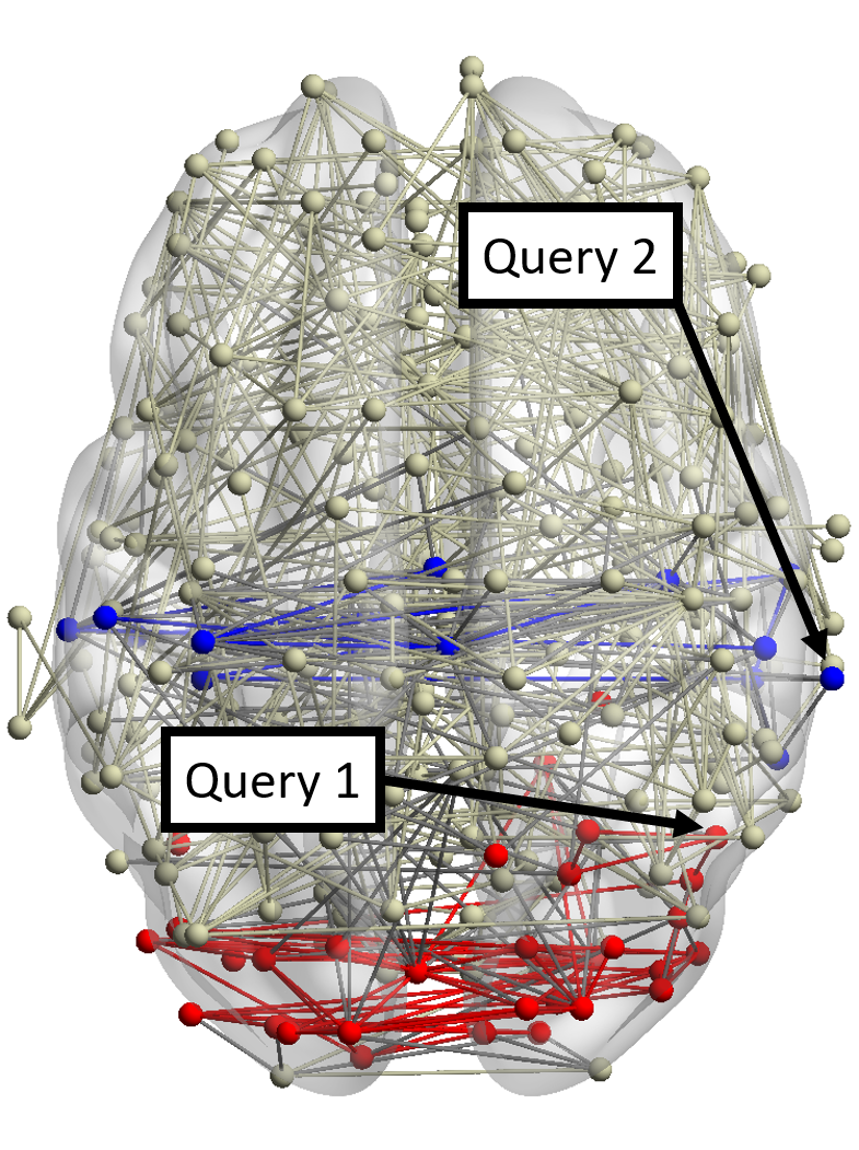
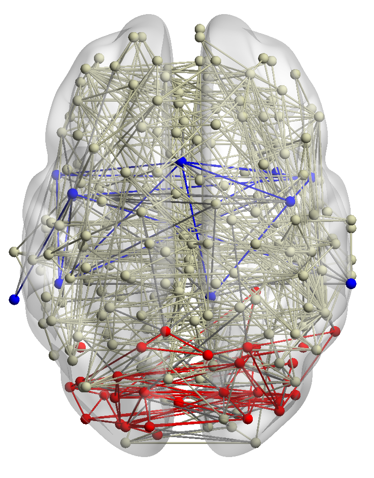
Case Study on the BrainNet Dataset. Detecting and monitoring functional systems in the human brain is an important task in
neuroscience. Brain networks can be built from neuroimages where nodes and edges are brain regions and their functional relations.
In many cases, however, the brain network generated from a single subject can be noisy and incomplete. Using brain networks
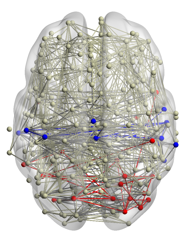
from many subjects helps to identify functional systems more accurately. For example, brain networks from three
subjects are shown in Fig. 5. Subjects 1 and 2 have similar visual conditions (red nodes); subjects 1 and 3 are with
similar auditory conditions (blue nodes). For a given query region, we want to find related regions with the same
functionality.
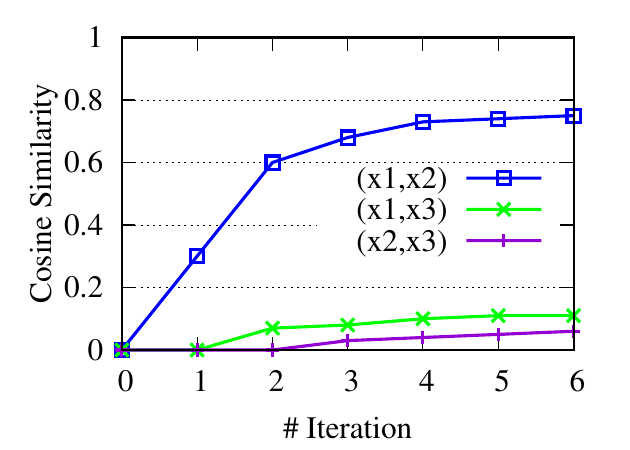
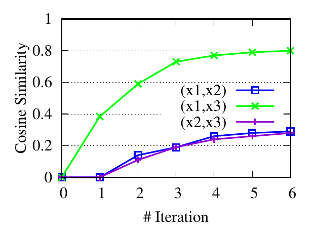
∙Detect relevant networks. To see whether RWM can automatically detect relevant networks, we run RWM model for Query 1 and
Query 2 in Fig. 5 separately. Fig. 6 shows the cosine similarity between the visiting probability vectors of different walkers along
iterations. x1, x2, and x3 are the three visiting vectors on the three brain networks, respectively. We see that the similarity between
the visiting histories of walkers in relevant networks, i.e., subjects 1 and 2 in Fig. 6(a), subjects 1 and 3 in 6(b), increases along with
the updating. But similarities in query-oriented irrelevant networks are very low during the whole process. This indicates
that RWM can actively select query-oriented relevant networks to help better capture the local structure for each
network.
∙Identify functional systems. In this case study, we further evaluate the detected results of RWM in the BrainNet
dataset. Note that other methods can only find a query-oriented local community in the network containing the query
node.
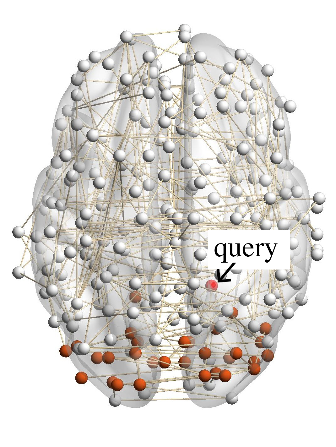
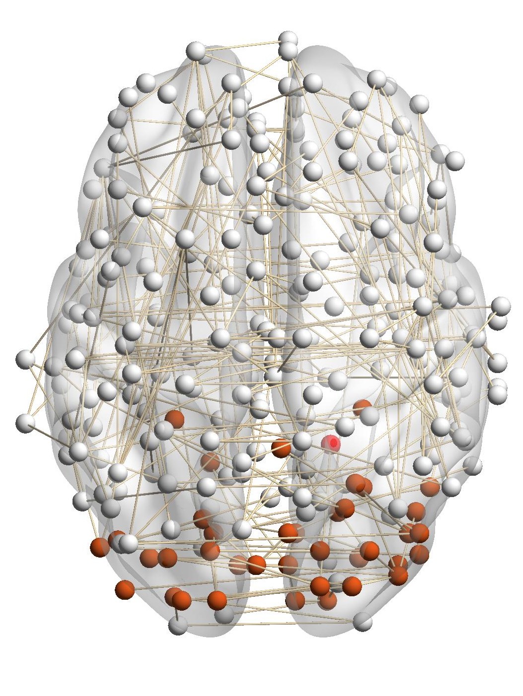
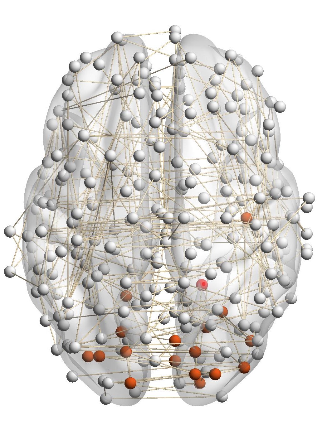
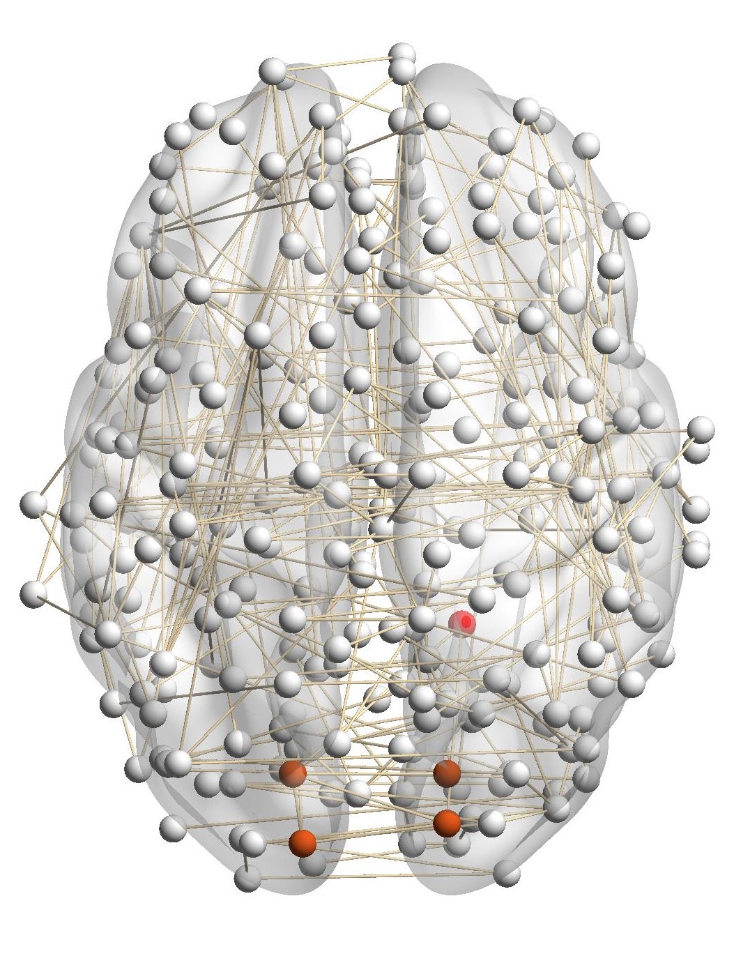
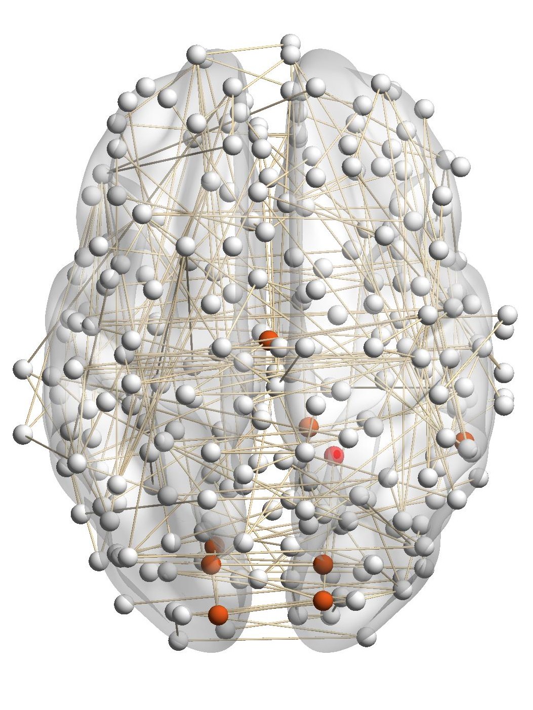
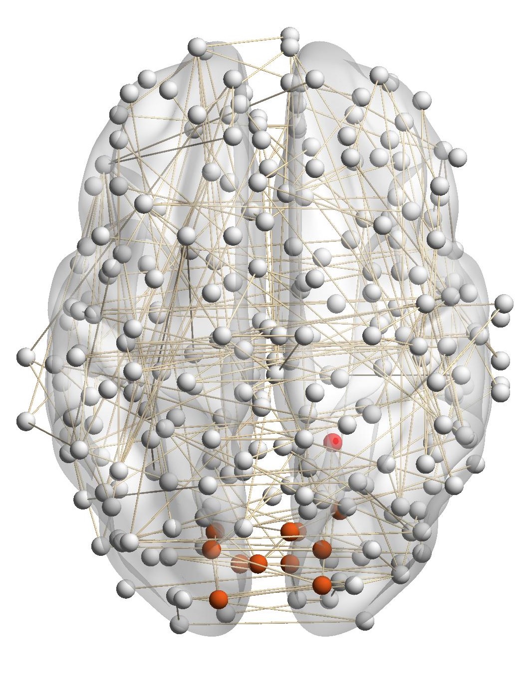
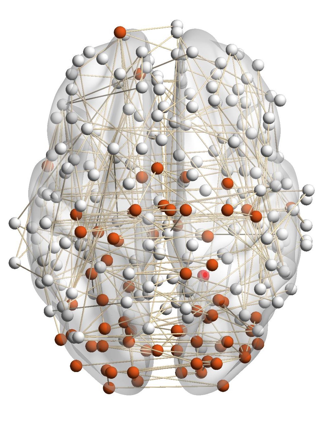
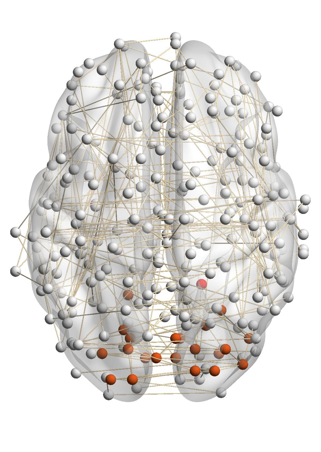
Figure 7(a) shows the brain network of a subject in the BrainNet dataset. The nodes highlighted in red represent the suggested
visual system of the human brain, which is used as the ground truth community. We can see that nodes in the visual system are not
only functionally related but also spatially close. We choose a node from the visual system as the query node, which is marked in
Figure 7(a). We apply our method as well as other baseline methods to detect the local community in the brain
network of this subject. The identified communities are highlighted in red in Figure 7. From Figure 7(b), we can see
that the community detected by our method is very similar to the ground truth. Single network methods, such as
RWR (Figure 7(c)), MWC (Figure 7(d)), LEMON (Figure 7(e)) and QDC (Figure 7(f)), suffer from the incomplete
information in the single network. Compared to the ground truth, they tend to find smaller communities. MRWR
(Figure 7(b)) includes many false positive nodes. The reason is that MRWR assumes all networks are similar and treat them
equally. ML-LCD (Figure 7(h)) achieves a relatively reasonable detection, while it still neglects nodes in the boundary
area.
Case Study on DBLP Dataset. In the general multiple networks, for a query node from one network, we only have the ground truth
local community in that network but no ground truth about the relevant local communities in other networks. So in this section, we
use DBLP as a case study to demonstrate the relevance of local communities detected from other networks by RWM. We use Prof.
Danai Koutra from UMich as the query. The DBLP dataset was collected in May 2014 when she was a Ph.D. student advised by Prof.
Christos Faloutsos. Table 4 shows the detected author community and paper community. Due to the space limitation,
instead of showing the details of the paper community, we list venues where these papers were published in. For
example, “KDD(3)” means that 3 KDD papers are included in the detected paper community. The table shows that our
method can detect local communities from both networks with high qualities. Specifically, the detected authors are
mainly from her advisor’s group. The detected paper communities are mainly published in Database/Data Mining
conferences.
Table 4
Case study on DBLP
|
|
| Author community | Paper community |
|
|
| Danai Koutra (query) | KDD (3) |
| Christos Faloutsos | PKDD (3) |
| Evangelos Papalexakis | PAKDD (3) |
| U Kang | SIGMOD (2) |
| Tina Eliassi-Rad | ICDM (2) |
| Michele Berlingerio | TKDE(1) |
| Duen Horng Chau | ICDE (1) |
| Leman Akoglu | TKDD (1) |
| Jure Leskovec | ASONAM (1) |
| Hanghang Tong | WWW(1) |
| ... | ... |
|
|
| |
6.3 Network Embedding
Network embedding aims to learn low dimensional representations for nodes in a network to preserve the network structure.
These representations are used as features in many tasks on networks, such as node classification [62], recommendation [52], and
link prediction [10]. Many network embedding methods consist of two components: one extracts contexts for nodes, and the other
learns node representations from the contexts. For the first component, random walk is a routinely used method to generate
contexts. For example, DeepWalk [46] uses the truncated random walk to sample paths for each node, and node2vec [15] uses
biased second order random walk. In this part, we apply the proposed RWM for the multiple network embedding. RM and Citeseer
are used in this part.
6.3.1 Experimental setup
To evaluate RWM on network embedding, we choose two classic network embedding methods: DeepWalk and
node2vec, and replace the first components (sampling parts) with RWM. We denote the DeepWalk and node2vec
with replacements by DeepWalk_RWM and node2vec_RWM respectively. Specifically, For each node on the target
network, RWM based methods first use the node as the starting node and calculate the static transition matrix of the
walker on the target network. Then truncated random walk (DeepWalk_RWM) and second order random walk
(node2vec_RWM) are applied on the matrix to generate contexts for the node. we compare these two methods with
traditional ones. Since we focus on the sampling phase of network embedding, to control the variables, for all four
algorithms, we use word2vec (skip-gram model) [36] with the same parameters to generate node embeddings from
sampling.
For all methods, the dimensionality of embeddings is 100. The walk length is set to 40 and walks per node is set to 10. For
node2vec, we use a grid search over p,q ∈{0.25,0.5,1,2,4} [15]. For RWM based methods, we set λ = 0.7,ϵ = 0.01,θ = 0.9.
Windows size of word2vec is set to its default value 5.
6.3.2 Accuracy Evaluation.
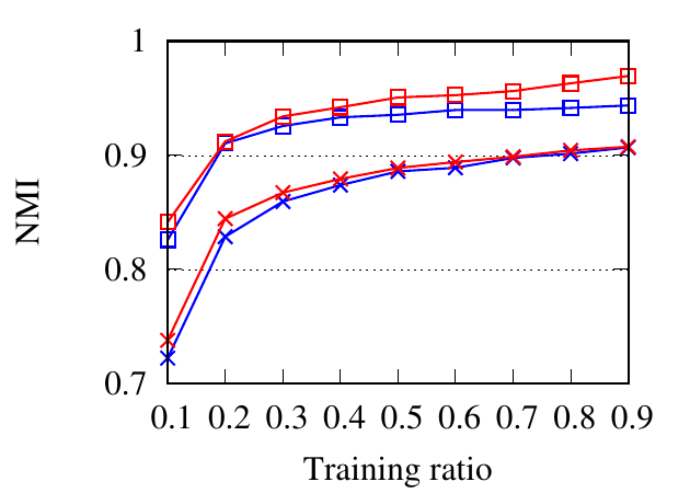
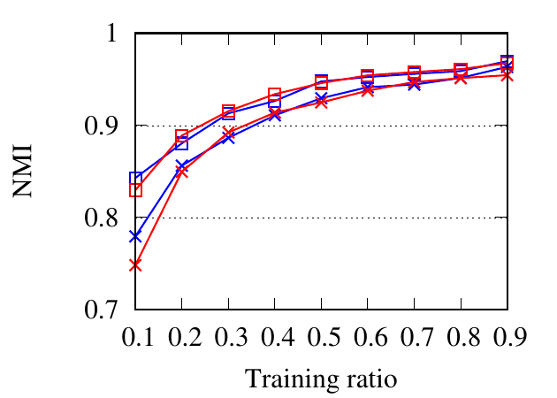
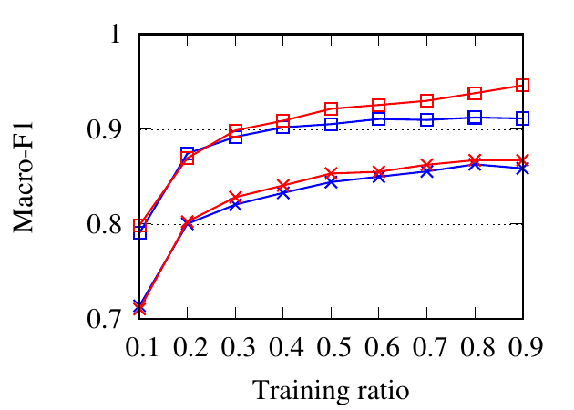
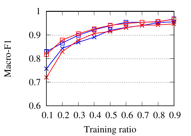
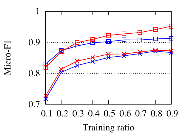
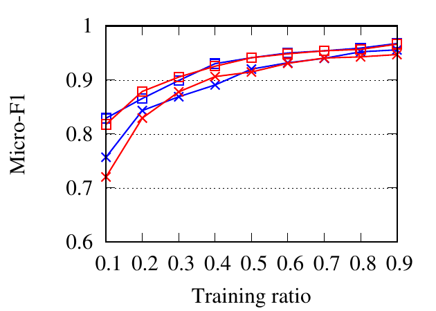
We compare different methods through a classification task. On each dataset, embedding vectors are learned from the full
dataset. Then the embeddings are used as input to the SVM classifier [45]. When training the classifier, we randomly sample a
portion of the nodes as the training set and the rest as the testing set. The ratio of training is varied from 10% to 90%. We use NMI,
Macro-F1, and Micro-F1 scores to evaluate classification accuracy. For RM, we set a network as the target network at one time
and report the average results here. For Citeseer, we only embed the collaboration network, since only authors are
labeled.
Fig. 8 shows the experimental results. RWM based network embedding methods consistently perform better than traditional
counterparts in terms of all metrics. This is because RWM can use additional information on multiple networks to refine node
embedding, while baseline methods are affected by noise and incompleteness on a single network. In most cases,
node2vec achieves better results than DeepWalk in both the traditional setting and RWM setting, which is similar to the
conclusion drawn in [15]. Besides, RWM based methods are much better than other methods in Citeseer dataset,
when the training ratio is small, e.g., 10%, which means RWM is more useful in real practice when the available
labels are scarce. This advantage comes from more information from other networks when embedding the target
network.
6.4 Link Prediction
We chose two multiplex networks, Genetic and Athletics to test our approach.
6.4.1 Experimental setup
Here we apply RWM based random walk with restart (RWR) on multiplex networks to calculate the proximity scores between
each pair of nodes on the target network, denoted by RWM. Then we choose the top 100 pairs of unconnected nodes with the
highest proximity scores as the predicted links. We compare this method with traditional RWR on the target networks, denoted by
Single, and RWR on the merged networks, which is obtained by summing up the weights of the same edges in all networks,
denoted by Merged. We choose the probability of restart α = 0.9 for all three methods and decay factor λ = 0.4 for
RWM.
We focus on one network, denoted by the target network, at one time. For the target network, we randomly remove 30% edges as
the probe edges, which are used as the ground truth for testing. Other networks are unchanged [32]. We use precision100 as the
evaluation measurement. The final results are averaged over all networks in the dataset.
6.4.2 Experimental Results
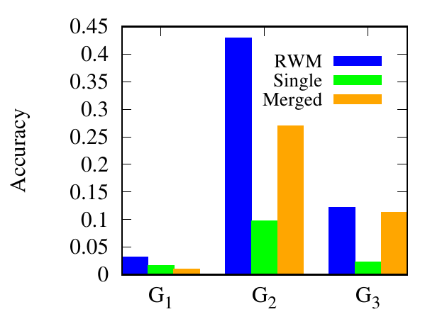
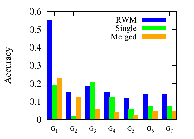
As shown in Fig. 9, for Athletics, our method consistently performs better than the other two methods. Specifically,
RWM based RWR outperforms the traditional RWR and RWR on the merged network by (93.37%, 218%) in G1,
(351.69%, 61.3%) in G2, (422.31%, 8.17%) in G3, in average, respectively. For Genetic, RWM based RWR achieves the best
results in 6 out of 7 networks. From the experimental results, we can draw a conclusion that using auxiliary link
information from other networks can improve link prediction accuracy. Single outperforms Merged in 1 out of 3 and 4
out of 7 networks in these two multiplex networks, respectively, which shows that including other networks does
not always lead to better results. Thus, RWM is an effective way to actively select useful information from other
networks.
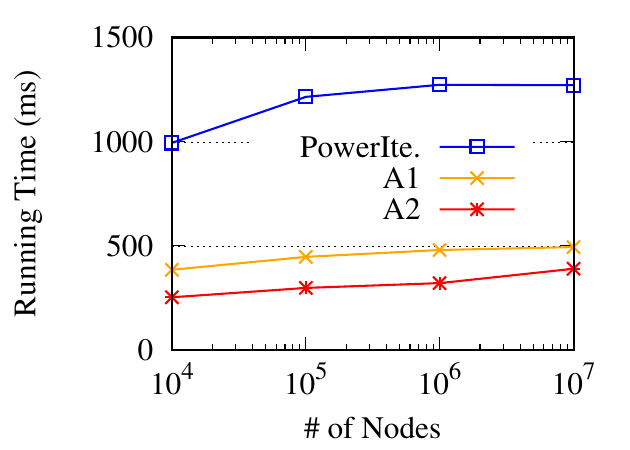
6.5 Efficiency Evaluation
Note that the running time of RWM using basic power-iteration (Algorithm 1) is similar to the iteration-based random walk local
community detection methods but RWM obtains better performance than other baselines with a large margin (Table 3). Thus, in this
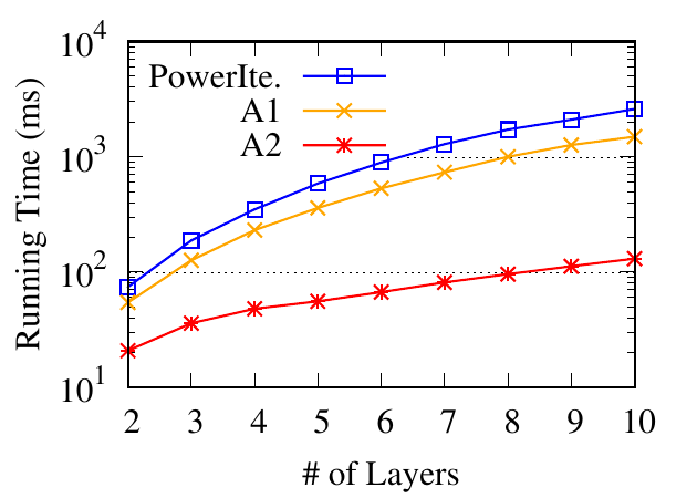
section, we focus on RWM and use synthetic datasets to evaluate its efficiency. There are three methods to update visiting
probabilities in RWM: (1) power iteration method in Algorithm 1 (PowerIte), (2) power iteration with early stopping introduced in
Sec. 4.1 (A1), and (3) partial updating in Sec. 4.2 (A2).
We first evaluate the running time w.r.t. the number of networks. We generate 9 datasets with different numbers of networks (2 to
10). For each dataset, we first use a graph generator [23] to generate a base network consisting of 1,000 nodes and about 7,000 edges.
Then we obtain multiple networks from the base network. In each network, we randomly delete 50% edges from the base network.
For each dataset, we randomly select a node as the query and detect local communities. In Fig. 10(a), we report the running
time of the three methods averaged over 100 trials. The early stopping in A1 saves time by about 2 times for the
iteration method. The partial updating in A2 can further speed up by about 20 times. Furthermore, we can observe
that the running time of A2 grows slower than PowerIte. Thus the efficiency gain tends to be larger with more
networks.
Next, we evaluate the running time w.r.t. the number of nodes. Similar to the aforementioned generating process, we synthesize 4
datasets from 4 base networks with the number of nodes ranging from 104 to 107. The average node degree is 7 in each base
network. For each dataset, we generate multiplex networks with three networks, by randomly removing half of the edges from the
base network. The running time is shown in Fig. 10(b). Compared to the power iteration method, the approximation methods are
much faster, especially when the number of nodes is large. In addition, they grow much slower, which enables their scalability on
even larger datasets.
We further check the number of visited nodes, which have positive visiting probability scores in RWM, in different-sized
networks. In Table 5, we show the number of visited nodes both at the splitting time Te and the end of updating (averaged over 100
trials). Note that we compute Te = ⌈log λ ⌉ according to Theorem 4 with K = 3,ϵ = 0.01,λ = 0.7. We see that in the end, only
a very small proportion of nodes are visited (for the biggest 107 network, probability only propagates to 0.02% nodes). This
demonstrates the locality of RWM. Besides, in the first phase (early stop at Te), visiting probabilities are restricted to about 50 nodes
around the query node.
⌉ according to Theorem 4 with K = 3,ϵ = 0.01,λ = 0.7. We see that in the end, only
a very small proportion of nodes are visited (for the biggest 107 network, probability only propagates to 0.02% nodes). This
demonstrates the locality of RWM. Besides, in the first phase (early stop at Te), visiting probabilities are restricted to about 50 nodes
around the query node.
Table 5
Number of visited nodes v.s. different network size
|
|
|
|
|
| | 104 | 105 | 106 | 107 |
|
|
|
|
|
| # visited nodes (Te) | 47.07 | 50.58 | 53.27 | 53.54 |
| # visited nodes (end) | 1977.64 | 2103.43 | 2125.54 | 2177.70 |
|
|
|
|
|
| |
7 Conclusion
In this paper, we propose a novel random walk model, RWM, on multiple networks. Random walkers on different networks sent
by RWM mutually affect their visiting probabilities in a reinforced manner. By aggregating their effects from local
subgraphs in different networks, RWM restricts walkers’ most visiting probabilities among the most relevant nodes.
Rigorous theoretical foundations are provided to verify the effectiveness of RWM. Two speeding-up strategies are also
developed for efficient computation. Extensive experimental results verify the advantages of RWM in effectiveness and
efficiency.
ACKNOWLEDGMENTS
This project was partially supported by NSF project IIS-1707548.
References
[1] M. Alamgir and U. Von Luxburg. Multi-agent random walks for local clustering on graphs. In ICDM, pages 18–27, 2010.
[2] R. Andersen, F. Chung, and K. Lang. Local graph partitioning using pagerank vectors. In FOCS, pages 475–486, 2006.
[3] N. Barbieri, F. Bonchi, E. Galimberti, and F. Gullo. Efficient and effective community search. Data mining and knowledge discovery,
29(5):1406–1433, 2015.
[4] Y. Bian, D. Luo, Y. Yan, W. Cheng, W. Wang, and X. Zhang. Memory-based random walk for multi-query local community detection.
Knowledge and Information Systems, pages 1–35, 2019.
[5] Y. Bian, J. Ni, W. Cheng, and X. Zhang. Many heads are better than one: Local community detection by the multi-walker chain. In
ICDM, pages 21–30, 2017.
[6] Y. Bian, J. Ni, W. Cheng, and X. Zhang. The multi-walker chain and its application in local community detection. Knowledge and
Information Systems, 60(3):1663–1691, 2019.
[7] Y. Bian, Y. Yan, W. Cheng, W. Wang, D. Luo, and X. Zhang. On multi-query local community detection. In ICDM, pages 9–18, 2018.
[8] A. Bojchevski, O. Shchur, D. Zügner, and S. Günnemann. Netgan: Generating graphs via random walks. In International conference on
machine learning, pages 610–619. PMLR, 2018.
[9] S. Cao, W. Lu, and Q. Xu. Grarep: Learning graph representations with global structural information. In CIKM, 2015.
[10] H. Chen, H. Yin, W. Wang, H. Wang, Q. V. H. Nguyen, and X. Li. Pme: projected metric embedding on heterogeneous networks for
link prediction. In SIGKDD, 2018.
[11] W. Cheng, X. Zhang, Z. Guo, Y. Wu, P. F. Sullivan, and W. Wang. Flexible and robust co-regularized multi-domain graph clustering.
In SIGKDD, pages 320–328. ACM, 2013.
[12] M. De Domenico, A. Lancichinetti, A. Arenas, and M. Rosvall. Identifying modular flows on multilayer networks reveals highly
overlapping organization in interconnected systems. Physical Review X, 5(1):011027, 2015.
[13] M. De Domenico, V. Nicosia, A. Arenas, and V. Latora. Structural reducibility of multilayer networks. Nature communications, 6:6864,
2015.
[14] M. Ghorbani, M. S. Baghshah, and H. R. Rabiee. Multi-layered graph embedding with graph convolutional networks. arXiv preprint
arXiv:1811.08800, 2018.
[15] A. Grover and J. Leskovec. node2vec: Scalable feature learning for networks. In SIGKDD, pages 855–864, 2016.
[16] R. Interdonato, A. Tagarelli, D. Ienco, A. Sallaberry, and P. Poncelet. Local community detection in multilayer networks. Data Mining
and Knowledge Discovery, 31(5):1444–1479, 2017.
[17] G. Jeh and J. Widom. Simrank: a measure of structural-context similarity. In KDD, pages 538–543, 2002.
[18] J. Kim and J.-G. Lee. Community detection in multi-layer graphs: A survey. ACM SIGMOD Record, 44(3):37–48, 2015.
[19] M. Kivelä, A. Arenas, M. Barthelemy, J. P. Gleeson, Y. Moreno, and M. A. Porter. Multilayer networks. Journal of complex networks,
2(3):203–271, 2014.
[20] J. Klicpera, A. Bojchevski, and S. Günnemann. Predict then propagate: Graph neural networks meet personalized pagerank. In ICLR,
2018.
[21] J. Klicpera, S. Weißenberger, and S. Günnemann. Diffusion improves graph learning. In NeurIPS, 2019.
[22] K. Kloster and D. F. Gleich. Heat kernel based community detection. In SIGKDD, pages 1386–1395, 2014.
[23] A. Lancichinetti and S. Fortunato. Benchmarks for testing community detection algorithms on directed and weighted graphs with
overlapping communities. Physical Review E, 2009.
[24] A. N. Langville and C. D. Meyer. Google’s PageRank and beyond: The science of search engine rankings. Princeton University Press, 2011.
[25] J. Leskovec and J. J. Mcauley. Learning to discover social circles in ego networks. In NIPS, pages 539–547, 2012.
[26] J. Li, C. Chen, H. Tong, and H. Liu. Multi-layered network embedding. In SDM, 2018.
[27] Y. Li, K. He, D. Bindel, and J. E. Hopcroft. Uncovering the small community structure in large networks: A local spectral approach. In
WWW, pages 658–668, 2015.
[28] K. W. Lim and W. Buntine. Bibliographic analysis on research publications using authors, categorical labels and the citation network.
Machine Learning, 103(2):185–213, 2016.
[29] R. Liu, W. Cheng, H. Tong, W. Wang, and X. Zhang. Robust multi-network clustering via joint cross-domain cluster alignment. In
ICDM, pages 291–300. IEEE, 2015.
[30] L. Lovász et al. Random walks on graphs: A survey. Combinatorics, Paul erdos is eighty, 2(1):1–46, 1993.
[31] D. Lu and H. Zhang. Stochastic process and applications. Tsinghua University Press, 1986.
[32] L. Lü, C.-H. Jin, and T. Zhou. Similarity index based on local paths for link prediction of complex networks. Physical Review E,
80(4):046122, 2009.
[33] D. Luo, J. Ni, S. Wang, Y. Bian, X. Yu, and X. Zhang. Deep multi-graph clustering via attentive cross-graph association. In WSDM,
pages 393–401, 2020.
[34] S. Ma, C. Gong, R. Hu, D. Luo, C. Hu, and J. Huai. Query independent scholarly article ranking. In ICDE, 2018.
[35] V. Martínez, F. Berzal, and J.-C. Cubero. A survey of link prediction in complex networks. ACM Computing Surveys, 2017.
[36] T. Mikolov, I. Sutskever, K. Chen, G. S. Corrado, and J. Dean. Distributed representations of words and phrases and their
compositionality. In NIPS, 2013.
[37] P. J. Mucha, T. Richardson, K. Macon, M. A. Porter, and J.-P. Onnela. Community structure in time-dependent, multiscale, and multiplex
networks. Science, 328(5980):876–878, 2010.
[38] P. J. Mucha, T. Richardson, K. Macon, M. A. Porter, and J.-P. Onnela. Community structure in time-dependent, multiscale, and multiplex
networks. science, 328(5980):876–878, 2010.
[39] M. E. Newman. Coauthorship networks and patterns of scientific collaboration. Proceedings of the national academy of sciences, 101(suppl
1):5200–5205, 2004.
[40] J. Ni, S. Chang, X. Liu, W. Cheng, H. Chen, D. Xu, and X. Zhang. Co-regularized deep multi-network embedding. In WWW, pages
469–478, 2018.
[41] J. Ni, W. Cheng, W. Fan, and X. Zhang. Comclus: A self-grouping framework for multi-network clustering. IEEE Transactions on
Knowledge and Data Engineering, 30(3):435–448, 2018.
[42] E. Omodei, M. D. De Domenico, and A. Arenas. Characterizing interactions in online social networks during exceptional events.
Frontiers in Physics, 3:59, 2015.
[43] L. Ou-Yang, H. Yan, and X.-F. Zhang. A multi-network clustering method for detecting protein complexes from multiple heterogeneous
networks. BMC bioinformatics, 2017.
[44] L. Page, S. Brin, R. Motwani, and T. Winograd. The pagerank citation ranking: Bringing order to the web. Technical report, Stanford
InfoLab, 1999.
[45] F. Pedregosa, G. Varoquaux, A. Gramfort, V. Michel, B. Thirion, O. Grisel, M. Blondel, P. Prettenhofer, R. Weiss, V. Dubourg,
J. Vanderplas, A. Passos, D. Cournapeau, M. Brucher, M. Perrot, and E. Duchesnay. Scikit-learn: Machine learning in Python. JMLR, 2011.
[46] B. Perozzi, R. Al-Rfou, and S. Skiena. Deepwalk: Online learning of social representations. In SIGKDD, 2014.
[47] J. Tang, M. Qu, M. Wang, M. Zhang, J. Yan, and Q. Mei. Line: Large-scale information network embedding. In WWW, pages 1067–1077,
2015.
[48] J. Tang, J. Zhang, L. Yao, J. Li, L. Zhang, and Z. Su. Arnetminer: extraction and mining of academic social networks. In SIGKDD, pages
990–998, 2008.
[49] H. Tong, C. Faloutsos, and J.-Y. Pan. Fast random walk with restart and its applications. In ICDM, pages 613–622, 2006.
[50] D. C. Van Essen, S. M. Smith, D. M. Barch, T. E. Behrens, E. Yacoub, K. Ugurbil, W.-M. H. Consortium, et al. The wu-minn human
connectome project: an overview. Neuroimage, 80:62–79, 2013.
[51] N. Veldt, C. Klymko, and D. F. Gleich. Flow-based local graph clustering with better seed set inclusion. In SDM, pages 378–386, 2019.
[52] Y. Wen, L. Guo, Z. Chen, and J. Ma. Network embedding based recommendation method in social networks. In WWW, 2018.
[53] Y. Wu, Y. Bian, and X. Zhang. Remember where you came from: on the second-order random walk based proximity measures.
Proceedings of the VLDB Endowment, 10(1):13–24, 2016.
[54] Y. Wu, R. Jin, J. Li, and X. Zhang. Robust local community detection: on free rider effect and its elimination. PVLDB, 8(7):798–809, 2015.
[55] Y. Wu, X. Zhang, Y. Bian, Z. Cai, X. Lian, X. Liao, and F. Zhao. Second-order random walk-based proximity measures in graph
analysis: formulations and algorithms. The VLDB Journal, 27(1):127–152, 2018.
[56] L. Xia, Y. Xu, C. Huang, P. Dai, and L. Bo. Graph meta network for multi-behavior recommendation. In Proceedings of the 44th
International ACM SIGIR Conference on Research and Development in Information Retrieval, pages 757–766, 2021.
[57] Y. Yan, Y. Bian, D. Luo, D. Lee, and X. Zhang. Constrained local graph clustering by colored random walk. In WWW, pages 2137–2146,
2019.
[58] Y. Yan, D. Luo, J. Ni, H. Fei, W. Fan, X. Yu, J. Yen, and X. Zhang. Local graph clustering by multi-network random walk with restart.
In PAKDD, pages 490–501, 2018.
[59] P. Yu, C. Fu, Y. Yu, C. Huang, Z. Zhao, and J. Dong. Multiplex heterogeneous graph convolutional network. In Proceedings of the 28th
ACM SIGKDD Conference on Knowledge Discovery and Data Mining, pages 2377–2387, 2022.
[60] H. Zhang and G. Kou. Role-based multiplex network embedding. In International Conference on Machine Learning, pages 26265–26280.
PMLR, 2022.
[61] W. Zhang, J. Mao, Y. Cao, and C. Xu. Multiplex graph neural networks for multi-behavior recommendation. In Proceedings of the 29th
ACM International Conference on Information & Knowledge Management, pages 2313–2316, 2020.
[62] W. Zhao, J. Zhu, M. Yang, D. Xiao, G. P. C. Fung, and X. Chen. A semi-supervised network embedding model for protein complexes
detection. In AAAI, 2018.


![(t+1) (t)
Δ (t+1)= ∥PiK - Pi ∥∞
= ∥∑ [Wˆ(t+1)(i,j) -Wˆ(t)(i,j)]P ∥
j=0 j ∞
∑ ˆ (t+1) ˆ(t)
= ∥j∈L[W (i,j)- W (i,j)]Pj
i∑ ˆ (t+1) ˆ (t)
+ ¯[W (i,j)- W (i,j)]Pj ∥∞
j∈Li](main8x.svg)
![Δ(t+ 1)= max{∥ ∑ [ ˆW (t+1)(i,j)- Wˆ(t)(i,j)]Pj ∥∞,
j∈Li
∥ ∑ [W ˆ(t+1)(i,j)-Wˆ (t)(i,j)]Pj ∥∞}
j∈¯Li](main11x.svg)
![∥ ∑ [ ˆW (t+1)(i,j)- Wˆ(t)(i,j)]P ∥
j∈Li j ∞
∑ W (t+1)(i,j) W (t)(i,j)
= ∥ [∑--W-(t+1)(i,k) - ∑-W-(t)(i,k)]Pj ∥∞
j∈Li k k
≤ ∥ ∑ [W∑-(t)(i,j)+-λt- ∑W--(t)(i,j)--]P ∥
j∈Li kW (t)(i,k) kW (t)(i,k) j ∞
∑ λt
≤ ∥ ∑--W-(t)(i,k)Pj ∥∞
j∑∈Li k
≤ ∥ λtPj ∥∞
j∈Li
≤λtK](main12x.svg)
![∥ ∑ [ ˆW (t+1)(i,j)- Wˆ(t)(i,j)]Pj ∥∞
j∈¯Li
∑ W (t)(i,j) W (t+1)(i,j)
= ∥ [∑--W-(t)(i,k) - ∑-W-(t+1)(i,k)]Pj ∥∞
j∈¯Li k k
= ∥ ∑ [∑-W-(t)(i,j)--
j∈¯Li kW (t)(i,k)
(t) (t+1) (t+1) (t+1)
- ∑W---(i,j)+-λ---cos(xi-(t+,1x)j(t)+1)-]Pj ∥∞
k W (t)(i,k)+λ(t+1)cos(xi ,xk )
t∑k cos(x(ti+1),x(kt+1))- ∑j ∈¯Licos(x(it+1),x(jt+1))
≤λ |-------------∑--W-(t)(i,k)--------------|
≤λtK k](main13x.svg)