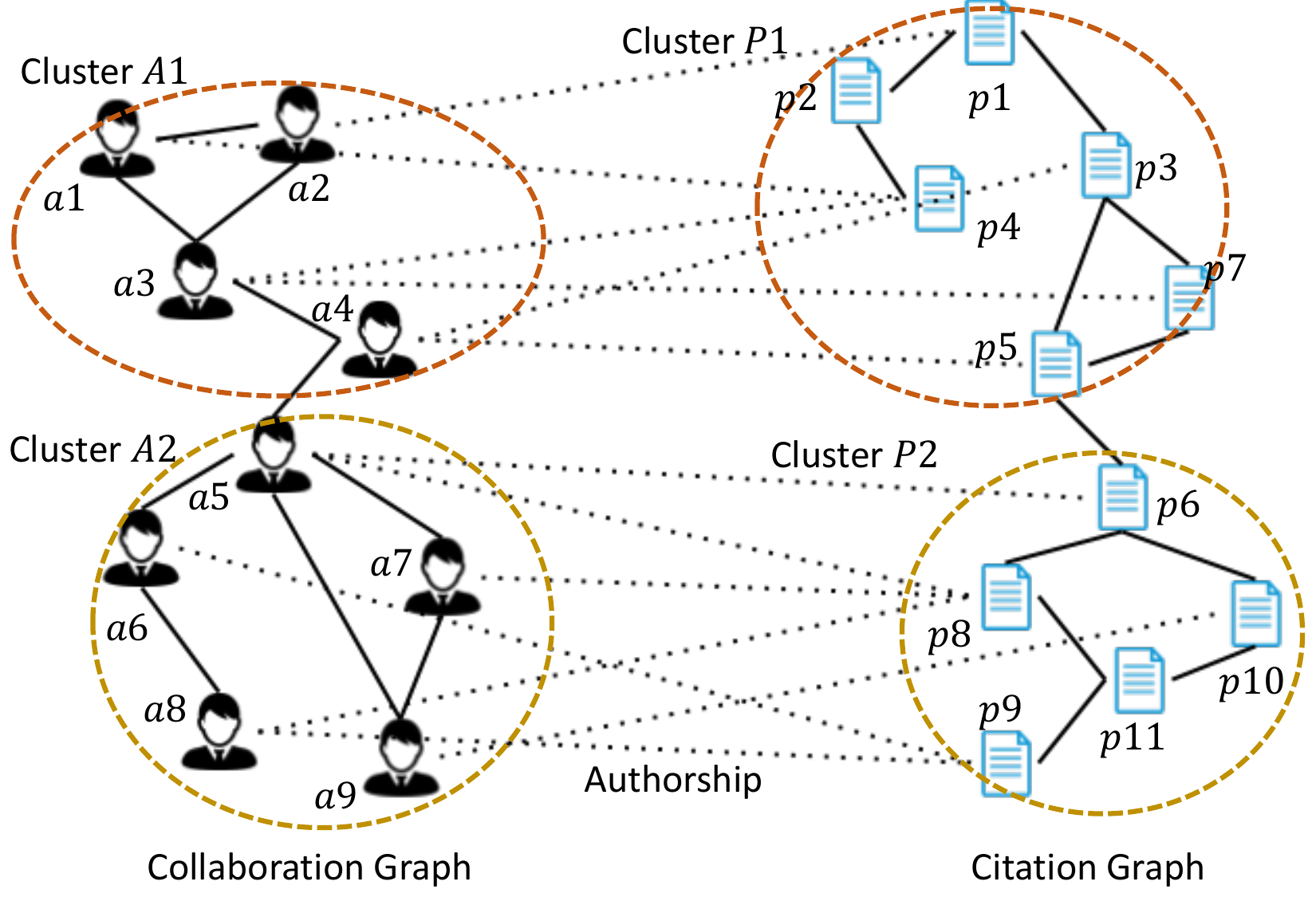
Figure 1: An illustrative example of multi-graph.
Deep Multi-Graph Clustering via Attentive Cross-Graph Association
Dongsheng Luo1, Jingchao Ni2, Suhang Wang1, Yuchen Bian3, Xiong Yu4, Xiang Zhang1
1Pennsylvania State University, 2NEC Labs America, 3Baidu Research, USA, 4Case Western Reserve University
{dul262,szw494,xzz89}@psu.edu,jni@nec-labs.com,yuchenbian@baidu.com,xxy21@case.edu
Multi-graph clustering aims to improve clustering accuracy by leveraging information from different domains, which has been shown to be extremely effective for achieving better clustering results than single graph based clustering algorithms. Despite the previous success, existing multi-graph clustering methods mostly use shallow models, which are incapable to capture the highly non-linear structures and the complex cluster associations in multi-graph, thus result in sub-optimal results. Inspired by the powerful representation learning capability of neural networks, in this paper, we propose an end-to-end deep learning model to simultaneously infer cluster assignments and cluster associations in multi-graph. Specifically, we use autoencoding networks to learn node embeddings. Meanwhile, we propose a minimum-entropy based clustering strategy to cluster nodes in the embedding space for each graph. We introduce two regularizers to leverage both within-graph and cross-graph dependencies. An attentive mechanism is further developed to learn cross-graph cluster associations. Through extensive experiments on a variety of datasets, we observe that our method outperforms state-of-the-art baselines by a large margin.
Graphs (or networks) are prevalent in real-life applications for modeling structured data such as social graphs [30], document citation graphs [19], and neurobiological graphs [27]. As a fundamental problem in graph analysis, graph clustering uncovers communities that are formed by densely connected nodes [13], which is widely used for understanding the underlying structure of a graph. Traditional methods, such as spectral clustering [29], modularity based clustering [18], and stochastic block model [16], are mostly developed for a single graph. The rapid growth of information in emerging applications, however, has generated a large volume of interdependent graphs, known as multi-graph, which necessitates clustering algorithms that enable joint consideration of multiple graphs and their in-between dependencies.
Fig. 1 illustrates an example of multi-graph, consisting of a collaboration graph on researchers and a citation graph on papers. Between the two graphs, an edge (i.e., the dotted line) indicates an authorship between a researcher and a paper. It is noteworthy that such cross-graph relationships establish the inter-dependency between the graphs thus are integral to any of their analysis. As another example, in neurobiology, brain networks are usually built to show the functional connectivity of the widespread brain regions by statistical analysis of the fMRI and other signals [27]. In a brain network, each node indicates a particular region and an edge represents functional connectivity between two regions. An emerging paradigm in neurobiology is that cognitive analysis is performed by jointly considering a collection of brain networks (of numerous subjects) instead of regarding each network in isolation [10]. In this scenario, the correspondence between the common regions in different networks establish the non-negligible inter-graph linkage in the collection of graphs.
Because of the increasingly growing volume of interdependent graphs on the web, substantial research attentions have been drawn to multi-graph clustering [2, 13, 20, 25]. Basically, the advantage of performing joint multi-graph clustering is two-fold. First, due to the measurement errors and data access limitations, in practice, individual graphs are often noisy and incomplete. In contrast, multi-graph provides complementary information to alleviate this problem, which is more robust. Exploiting it is a promising approach for revealing the authentic manifold structures so as to enhance clustering accuracy. Second, as a unique characteristic of multi-graph data, the cross-graph links will enable the discovery of new patterns that cannot be found in individual graphs. One such important pattern is the hidden association that may be exhibited between clusters from different graphs, which is essential to a comprehensive understanding of the entire system. For instance, a cluster of researchers (e.g., cluster A1 in Fig. 1) may publish a cluster of papers sharing similar topics (e.g., cluster P1 in Fig. 1), which may only be depicted by the cluster-level associations. Meanwhile, correctly identifying cluster associations will facilitate the establishment of clear boundaries between clusters within each graph, thus enhance clustering accuracy. For example, over a set of brain networks, a tight association of the visual systems (i.e., clusters of visual regions) will reduce the chance that a particular visual region deviates from its cluster in an individual brain network.
Despite the aforementioned advantages, multi-graph clustering remains a challenging task. First, recent intensive researches on graph representation learning have demonstrated that graph data are complex with highly non-linear underlying structures [31]. Hence it is important to take the potential non-linearity of the data into account when doing graph clustering. Whereas, how to model the non-linear hidden representations in the meantime of clustering graphs is still an open problem till now. Second, interdependent graphs may have quite different topological properties. For example, one graph is dense while another is sparse. Thus it is challenging to maintain the respective structures of individual graphs while leveraging the consistency. Finally, although inter-graph links are available at node-level, how to correctly infer the hidden cluster associations and use them for reinforcing the clustering accuracy is non-trivial, especially considering the inter-graph links are often scarce with the presence of noise.
To address the above challenges, in this work, we keep abreast of the ongoing developments of graph neural networks [7, 9, 28, 31] and pertinent AI techniques [8], and propose a novel algorithm DMGC, (Deep Multi-Graph Clustering), based on a deep learning model with a neural attention mechanism. Our goal is to seamlessly perform the dual procedures of multi-graph clustering and cross-graph cluster association, for improving clustering accuracy and interpreting cluster associations. Specifically, DMGC maps nodes to non-linear latent spaces via an autoencoding architecture [31] that preserves the 1st and 2nd order proximities between nodes in individual graphs. It manipulates the deep representations of nodes in the manifolds of multiple graphs via a minimum-entropy based clustering loss, which models nodes and cluster centroids by Cauchy distribution [36] and ensures tight and well-bounded clusters. In the meantime, DMGC infers associations between cluster centroids (i.e., the agents of clusters) over different graphs by a new attention mechanism. To preserve the autonomy of the topological properties of individual graphs, DMGC allows each graph to have its own latent space, while defines attention based functions to project cluster centroids from a unified space to the latent spaces of different graphs. Different from many existing deep learning based methods [26], which alternately perform representation learning and graph clustering, DMGC is a completely end-to-end clustering model that is pretrain-free. Our contributions are summarized as follows.
We propose to investigate the joint problem of deep multi-graph clustering and cross-graph cluster association, which is entirely unsupervised thus is very challenging.
We propose the first deep learning based multi-graph clustering methods, DMGC, which is an end-to-end model with an attention module to associate clusters across graphs.
We develop a new minimum-entropy based loss for graph clustering and a new attentive module for inferring cross-graph cluster associations.
We perform extensive experiments on a variety of real-life datasets. The results demonstrate that DMGC outperforms the-state-of-the-art methods by a large margin.
Traditional graph clustering methods are mostly designed for a single graph, such as spectral clustering [17], matrix factorization [11], modularity based clustering [18], and cut-based methods [3]. Recently, to tackle the highly nonlinear structures, various deep learning methods have been proposed [1, 22, 26, 34, 37]. In [26], GraphEncoder is used to learn node embeddings. K-means is then applied to get the clustering results. Several end-to-end models are also proposed [1, 22, 34, 37]. In [37], graph clustering are discussed in a supervised setting. Limited ground-truth clusters are utilized to learn an embedding model that is aware of the underlying social patterns. In [34], a unified modularized non-negative matrix factorization model is proposed to incorporate both node features and community structure for network embedding. In [22], the authors extend Deepwalk [21] by adding a cluster constraint. All the above methods are designed for a single graph and cannot handle multi-graph data.
Recently, multi-graph has drawn increasing attention because of its capability to model structural data from different domains [4, 12, 19, 20, 25, 32]. Various graph mining tasks have been extended to multi-graph setting, including the ranking problem [32], network embedding [4, 12, 19], and node clustering [2, 13, 20, 25]. Specifically, in [25], the authors propose linked matrix factorization method to achieve consensus clustering results among multiple graphs. This work is designed for a special type of multi-graph where all graphs share the same set of nodes. In [2], matrix factorization is extended to capture the inter-graph relationship by introducing the residual sum of square loss function and clustering disagreement loss function. In [13], the authors combine matrix tri-factorization with a cluster alignment loss. In [20], a probability model is proposed to detect the shared underlying clustering patterns of different graphs. However, these matrix factorization based methods and other shallow models may not be effective to capture the complex underlying patterns of multi-graph.
Suppose we have 𝑔 graphs, each is represented by 𝐺(𝑖)= (V(𝑖),E(𝑖)) (1 ≤𝑖≤𝑔), where V(𝑖) and E(𝑖) are the sets of nodes and edges in the graph, respectively. A(𝑖)∈R+𝑛𝑖×𝑛𝑖 is the adjacency matrix of 𝐺(𝑖), where 𝑛𝑖= |V(𝑖)|. Our analysis applies to any (un)directed and (un)weighted graphs. Thus A(𝑖) can be either symmetric or asymmetric, with binary or continuous entries. We use I = {(𝑖,𝑗)} to denote the set of available inter-graph dependencies. For instance, I = {(1,2),(2,3)} specifies two inter-graph dependencies, one is between 𝐺(1) and 𝐺(2), and another is between 𝐺(2) and 𝐺(3). Each pair (𝑖,𝑗) is coupled with a matrix S(𝑖𝑗)∈R+𝑛𝑖×𝑛𝑗, with 𝑠𝑥𝑦(𝑖𝑗) indicating the weight between node 𝑥 in 𝐺(𝑖) and node 𝑦 in 𝐺(𝑗). For clarity, important notations are summarized in Table 1.
Given {A(𝑖)}𝑖=1𝑔, {S(𝑖𝑗)}(𝑖,𝑗)∈I, and {𝐾𝑖}𝑖=1𝑔, where 𝐾𝑖 is the number of clusters in 𝐺(𝑖), the goal of this work is two-fold. First, for each node 𝑥 in each 𝐺(𝑖), we infer a cluster assignment probability q𝑥(𝑖)∈R+𝐾𝑖, with 𝑞𝑥𝑘(𝑖) measuring the probability that node 𝑥 belongs to cluster 𝑘 (1 ≤𝑘≤𝐾𝑖). Second, for each cluster 𝑘 in 𝐺(𝑖), we infer a cluster association probability c𝑘(𝑖𝑗)∈R+𝐾𝑗, with 𝑐𝑘𝑙(𝑖𝑗) measuring the probability that cluster 𝑘 in 𝐺(𝑖) associates with cluster 𝑙 in 𝐺(𝑗) (1 ≤𝑙≤𝐾𝑗), for any 𝑗 s.t. (𝑖,𝑗)∈I . We will demonstrate that, by jointly solving this dual task, the clustering performance will be significantly improved in Sec. 5.
| Symbol | Definition
|
| V(𝑖), E(𝑖) | the node/edge set of 𝑖-th graph |
| 𝑛𝑖 | the number of nodes in the 𝑖-th graph |
| A(𝑖) | the adjacency matrix of the 𝑖-th graph |
| Q(𝑖) | the cluster assignment matrix for the 𝑖-th graph |
| 𝐾𝑖 | the number of clusters of the 𝑖-th graph |
| 𝝁𝑘(𝑖) | the 𝑘-th cluster centroid of the 𝑖-th graph |
| H(𝑖) | the hidden representations of nodes in the 𝑖-th graph |
| 𝑑𝑖 | the embedding size of nodes in graph 𝐺(𝑖) |
| z𝑘(𝑖) | the 𝑘-th cluster centroid of 𝐺(𝑖) in the unified space. |
| 𝑔 | the number of graphs |
| I | the set of available cross-graph relationships. |
| S(𝑖𝑗) | the relationship matrix between nodes in 𝐺(𝑖) and 𝐺(𝑗) |
| C(𝑖𝑗) | the association matrix between clusters in 𝐺(𝑖) and 𝐺(𝑗) |
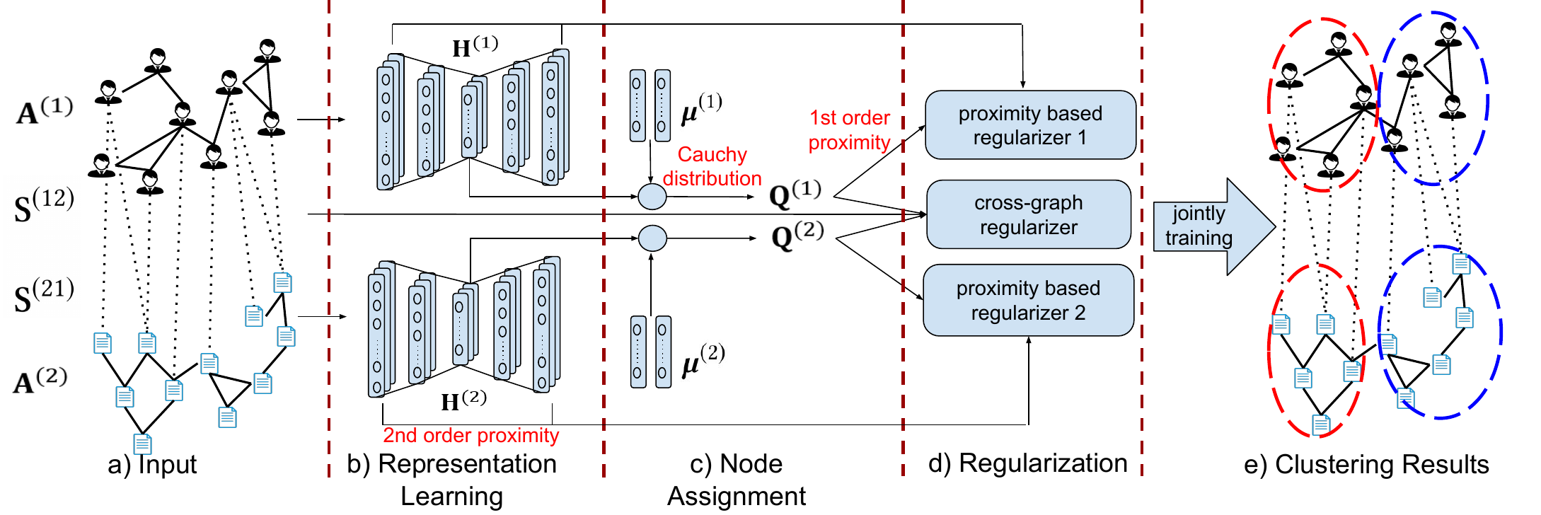
In this section, we introduce the DMGC method. Fig. 2 illustrates the architecture of DMGC for two interdependent graphs. First, each graph is fed to an autoencoding component to learn node embeddings that preserve the proximity between nodes in the graphs. Meanwhile, for each graph, node embeddings are assigned to cluster centroids (i.e., 𝝁(𝑖)) via measuring a Cauthy distribution. The probabilities of cluster membership (i.e., q𝑥(𝑖)) of different graphs are then regularized by a within-graph local proximity loss and a cross-graph cluster association loss. DMGC associates the cluster centroids of different graphs by an attention mechanism, where the learned attention weight specifies the relationship between clusters of different graphs. Finally, a joint loss is trained for obtaining the clustering results and attention weights. Next, we first introduce a novel clustering loss based on node embeddings.
4.1 Minimum-Entropy Based Clustering. Suppose we have already transformed each node 𝑥 in graph 𝐺(𝑖) (1 ≤𝑖≤𝑔) to its latent embedding. Let the embedding be h𝑥(𝑖)∈R1×𝑑𝑖, where 𝑑𝑖 is the dimensionality of the embedding space of 𝐺(𝑖), which can be different for different 𝑖’s. In addition, for each cluster 𝑘 in 𝐺(𝑖), we associate it with a centroid vector 𝝁𝑘(𝑖)∈R1×𝑑𝑖. Later in Sec. 4.3, we will discuss our approach to learn 𝝁𝑘(𝑖)’s by an attention based projection. For now, we use them to define a minimum-entropy based clustering loss.
To measure the similarity between h𝑥(𝑖) and the 𝑘-th cluster centroid 𝝁𝑘(𝑖), we employ the Cauchy distribution as a kernel function. As discussed in [14], comparing to Gaussian kernel, a model based on Cauchy distribution is more effective to force h𝑥(𝑖) apart from the centroid 𝝁𝑘(𝑖) if 𝑥 does not belong to cluster 𝑘, which implies a larger boundary. Therefore, we define a score 𝑞𝑥𝑘(𝑖) to indicate the probability that node 𝑥 belongs cluster 𝑘 by
| (1) |
Ideally, an uneven distribution q𝑥(𝑖)= [𝑞𝑥1(𝑖),...,𝑞𝑥𝐾𝑖(𝑖)] is highly desirable such that 𝑞𝑥𝑘(𝑖) is clearly distinguishable from 𝑞𝑥𝑘′(𝑖) (𝑘′≠ 𝑘) if 𝑥 belongs to cluster 𝑘. One option is to minimize the entropy of q𝑥(𝑖), which facilitates to resolve the uncertainty of a distribution [23]. Formally, the entropy of q𝑥(𝑖) is defined as
| (2) |
Since 𝑥log 𝑥 is convex and non-positive for 0 <𝑥<1, we have

where the equality holds if and only if q𝑥 is a one-hot vector, with 𝑞𝑥𝑘(𝑖)= 1 indicating node 𝑥 belongs to cluster 𝑘 with probability 1. Therefore, by minimizing 𝐻(q𝑥 (𝑖) ), we tend to achieve a sharp distribution q𝑥(𝑖) as a clear indicator of cluster membership.
However, minimizing entropy may cause the gradient exploding problem during the training with gradient descent. Specifically,
 |
Hence, when 𝑞𝑥𝑘(𝑖)→0, the above gradient tends to be very large which will dominate the gradient of the final loss and result in unstable results. To solve this issue, instead of minimizing Eq. (2), we introduce an inner product based loss
| (3) |
where σ(·) denotes the sigmoid function. Since 0 ≤𝑞𝑥𝑘(𝑖)≤1 and ∑ 𝑘𝑞𝑥𝑘(𝑖)= 1, we have
 |
where the equality holds when q𝑥 is a one-hot vector with 𝑞𝑥𝑘(𝑖)= 1, which shows that Eq. (2) and Eq. (3) have the same optimal solution. Also, it is worth to note that
 |
which solves the issue caused by gradient exploding.
Furthermore, to circumvent the trivial solution when all nodes are
assigned to a single cluster, we define an empirical distribution
𝑝𝑘(𝑖)=  ∑
𝑥𝑞𝑥𝑘(𝑖), which can be considered as the soft frequency of
each cluster. Then we minimize KL(p(𝑖)||u(𝑖)), the KL divergence
between p(𝑖) and the uniform prior u(𝑖), so as to to achieve a
balanced clustering. Consequently, our clustering loss for all graphs
becomes
∑
𝑥𝑞𝑥𝑘(𝑖), which can be considered as the soft frequency of
each cluster. Then we minimize KL(p(𝑖)||u(𝑖)), the KL divergence
between p(𝑖) and the uniform prior u(𝑖), so as to to achieve a
balanced clustering. Consequently, our clustering loss for all graphs
becomes
| (4) |
4.2 Proximity Based Constraints. Next, we discuss the 1st and 2nd order proximity based constraints to further refine our clustering quality. The 1st Order Proximity. Intuitively, two connected nodes are more likely to be assigned to the same cluster. Therefore, the 1st order proximity is introduced to capture the local graph structure through pairwise similarity between nearby nodes. Because our goal is clustering, instead of preserving the proximity via node embeddings as many existing works have done [6, 7, 19, 21, 31], we preserve the 1st order proximity by using the clustering vector q𝑥(𝑖). Formally, we minimize the following loss
| (5) |
where E(𝑖) is the set of edges in 𝐺(𝑖). By minimizing 𝐿1𝑠𝑡(𝑖), node 𝑥 and node 𝑦 tend to clustered together if they are linked in 𝐺(𝑖).
The 2nd Order Proximity. Moreover, as demonstrated by [31], preserving the 2nd order proximity is useful to encode the graph structure beyond pairwise similarity. Basically, this proximity measures the similarity between the neighborhoods of nodes. Let a𝑥(𝑖)∈R1×𝑛𝑖 be the adjacency vector of node 𝑥, i.e., the 𝑥-th row of the adjacency matrix A(𝑖). Thus, a𝑥(𝑖) encodes the neighborhood of node 𝑥. To preserve the 2nd order proximity, we perform the following transformation based on a𝑥(𝑖)
| (6) |
where 𝑓𝜽1(𝑖)(𝑖)(·) is an encoding function parameterized by 𝜽1(𝑖),
𝑔𝜽2(𝑖)(𝑖)(·) is a decoding function parameterized by 𝜽2(𝑖), and  𝑥(𝑖) is
a reconstruction of a𝑥(𝑖). Here, 𝑓𝜽1(𝑖)(𝑖)(·) and 𝑔𝜽2(𝑖)(𝑖)(·) can be
realized by different options, such as the fully connected network (FC)
and LSTM. In this work, we choose FC for its good performance in our
experiments.
𝑥(𝑖) is
a reconstruction of a𝑥(𝑖). Here, 𝑓𝜽1(𝑖)(𝑖)(·) and 𝑔𝜽2(𝑖)(𝑖)(·) can be
realized by different options, such as the fully connected network (FC)
and LSTM. In this work, we choose FC for its good performance in our
experiments.
Let h𝑥(𝑖)= 𝑓θ1(𝑖)(𝑖)(a𝑥(𝑖)) be the embedding of node 𝑥, as
introduced in Eq. (1). Since the adjacency vector encodes the
neighborhood of a node, minimizing the reconstruction error between
 𝑥(𝑖) and a𝑥(𝑖) will enforce nodes with similar neighborhood to have
similar embeddings. Hence, the 2nd order proximity can be preserved
in the embedding space by minimizing
𝑥(𝑖) and a𝑥(𝑖) will enforce nodes with similar neighborhood to have
similar embeddings. Hence, the 2nd order proximity can be preserved
in the embedding space by minimizing
| (7) |
where V(𝑖) is the set of nodes in 𝐺(𝑖), and ⊙ is the element-wise product. Here, similar to [31], we introduce a weight vector b𝑥(𝑖) to place more attention on the non-zero elements in a𝑥(𝑖) so as to handle the sparsity in a𝑥(𝑖). In particular, 𝑏𝑥𝑦(𝑖)= 𝑏>1 if 𝑎𝑥𝑦(𝑖)>0; 𝑏𝑥𝑦(𝑖)= 1 otherwise. In this paper, we empirically set 𝑏= 3.
Finally, putting Eq. (5) and Eq. (7) together, we achieve a proximity based loss
| (8) |
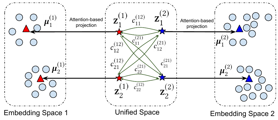
4.3 Cross-Graph Cluster Association. In this section, we develop an attention based method to model the association between clusters across different graphs.
In Eq. (1), we have introduced a cluster centroid 𝝁𝑘(𝑖) for each cluster 𝑘 in each 𝐺(𝑖). First, we discuss how to infer 𝝁𝑘(𝑖)’s. To preserve the autonomy of individual graphs, 𝝁𝑘(𝑖)’s are defined in different embedding spaces for different 𝐺(𝑖)’s, which may have different dimensionality 𝑑𝑖’s. This discrepancy hinders comparison between the centroids of different graphs. To solve it, we define a unified space particularly for all cluster centroids from all graphs. As illustrated in Fig. 3, in this space, each centroid is represented by a vector z𝑘(𝑖)∈R1×𝑑 with a uniform dimensionality 𝑑, which facilitates comparison. Then, to generate 𝝁𝑘(𝑖) in individual embedding spaces, we perform a projection from the unified space to the embedding space of each graph by an attention based single-layer FC
| (9) |
where 𝑐𝑘𝑙(𝑖𝑗) is an attention weight measuring the association between cluster centroid 𝑘 in 𝐺(𝑖) and cluster centroid 𝑙 in 𝐺(𝑗). [·; ·] represents a concatenation function. W(𝑖) is the weight of FC. Note in Eq. (9), the concatenation excludes the term for within-graph attention ∑ 𝑙𝑐𝑘𝑙(𝑖𝑖)z𝑙(𝑖).
By concatenating all centroids from all graphs other than 𝐺(𝑖) (via attention weights) together with z𝑘(𝑖), the output 𝝁𝑘(𝑖) is able to capture cross-graph dependencies at the cluster-level.
To define the attention 𝑐𝑘𝑙(𝑖𝑗), for the same reason as Eq. (1), we employ Cauchy distribution as the kernel to measure the associations between clusters in different graphs
| (10) |
For example, Fig. 3 shows the attention weights between the cluster centroids from two graphs in the unified space. The attention weights are directional, so both 𝑐11(12) and 𝑐11(21) exist between the 1st cluster in 𝐺(1) and the 1st cluster in 𝐺(2). To our best knowledge, this is the first work to model the hidden cross-graph cluster association by neural attention mechanism.
4.4 Cross-Graph Regularization. Next, we discuss on how to leverage the inter-graph links for clustering by using the attention weights in Eq. (10). Recall that the cluster assignment distribution of a node 𝑥 in graph 𝐺(𝑖) is q𝑥(𝑖). Intuitively, if 𝑥 is strongly linked to a node 𝑦 in 𝐺(𝑗), then the cluster of 𝑥 and the cluster of 𝑦 are likely to be associated, i.e., 𝑐𝑘𝑙(𝑖𝑗) is large, if the two clusters are denoted by 𝑘 and 𝑙. More generally, let C(𝑖𝑗)∈R𝐾𝑖×𝐾𝑗 be an attention matrix whose (𝑘,𝑙)-th entry is 𝑐𝑘𝑙(𝑖𝑗). Then this intuition implies the two vectors q𝑥(𝑖) and q𝑦(𝑗)(C(𝑖𝑗))𝑇 are similar in certain metric. Now we generalize this relationship to the case when 𝑥 links to multiple nodes in 𝐺(𝑗). Let N𝑥(𝑖→𝑗) be the set of nodes in 𝐺(𝑗) that are linked to 𝑥 in 𝐺(𝑖) with positive weights. To penalize the inconsistency of clustering assignments, we propose the following loss function.
| (11) |
where
| (12) |
and 𝑠𝑥𝑦(𝑖𝑗) is the weight on the inter-graph link between 𝑥 in 𝐺(𝑖) and 𝑦 in 𝐺(𝑗). Here, q𝑥(𝑖→𝑗) specifies a transferred clustering probability of node 𝑥, through node 𝑦’s that belong to N𝑥(𝑖→𝑗).
Let S(𝑖𝑗)∈R+𝑛𝑖×𝑛𝑗 be a matrix with the (𝑥,𝑦)-th entry as 𝑠𝑥𝑦(𝑖𝑗),
we perform a row-normalization on it to obtain  (𝑖𝑗). Then, by
summing up Eq. (11) over all nodes in all graphs, we have the
following loss function for cross-graph regularization.
(𝑖𝑗). Then, by
summing up Eq. (11) over all nodes in all graphs, we have the
following loss function for cross-graph regularization.
| (13) |
where we introduce a diagonal matrix O(𝑖𝑗)∈{0,1}𝑛𝑖×𝑛𝑖, with
𝑜𝑥𝑥(𝑖𝑗)= 0 if the 𝑥-th row of  (𝑖𝑗) is all-zero; and 𝑜𝑥𝑥(𝑖𝑗)= 1
otherwise.
(𝑖𝑗) is all-zero; and 𝑜𝑥𝑥(𝑖𝑗)= 1
otherwise.
4.5 Objective Function and Algorithm. Now, we can integrate the clustering loss in Eq. (4), the proximity loss in Eq. (8), and the cross-graph regularizer in Eq. (13) into a unified objective function
| (14) |
where 𝚯 = {𝜽1 (1) , 𝜽2 (1) , ...𝜽2 (𝑔) } are parameters of the autoencoder (Eq. (6)), Z= {Z(1),...,Z(𝑔)} are cluster centroids in the unified space (Eq. (10)), and W = {W(1),...,W(𝑔)} are the parameters of the FC networks for attention based centroid projection (Eq. (9)). α and β are hyper-parameters for trade-off between different loss components. Later in Sec. 5.5, we will evaluate the impacts of α and β to demonstrate the importance of 𝐿𝑝𝑟𝑜𝑥𝑖𝑚𝑖𝑡𝑦 and 𝐿𝑐𝑟𝑜𝑠𝑠.
 (𝑖𝑗)}(𝑖,𝑗)∈I, and α, β
Output: Cluster assignments {Q(𝑖)}𝑖=1𝑔 and cluster associations
{C(𝑖𝑗)}(𝑖,𝑗)∈I.
1Initialize parameters Θ, W, clusters centroids Z;
2while not convergence do
3
4
5Compute {Q(𝑖)}𝑖=1𝑔 by Eq. (1);
6Compute {C(𝑖𝑗)}(𝑖,𝑗)∈Iby Eq. (10);
7Compute loss the 𝐿by Eq. (14) ;
8Update Θ, W, and Zby minimizing 𝐿using Adam;
9return {Q(𝑖)}𝑖=1𝑔, {C(𝑖𝑗)}(𝑖,𝑗)∈I.__________________________________________________________
(𝑖𝑗)}(𝑖,𝑗)∈I, and α, β
Output: Cluster assignments {Q(𝑖)}𝑖=1𝑔 and cluster associations
{C(𝑖𝑗)}(𝑖,𝑗)∈I.
1Initialize parameters Θ, W, clusters centroids Z;
2while not convergence do
3
4
5Compute {Q(𝑖)}𝑖=1𝑔 by Eq. (1);
6Compute {C(𝑖𝑗)}(𝑖,𝑗)∈Iby Eq. (10);
7Compute loss the 𝐿by Eq. (14) ;
8Update Θ, W, and Zby minimizing 𝐿using Adam;
9return {Q(𝑖)}𝑖=1𝑔, {C(𝑖𝑗)}(𝑖,𝑗)∈I.__________________________________________________________
Time Complexity. Let the number of epochs be ℓ. Since the dimensionality of each embedding space 𝑑𝑖 is often much smaller than 𝑛𝑖, we can regard it as a constant. Let 𝑚𝑖𝑗 be the number of cross-graph edges between 𝐺(𝑖) and 𝐺(𝑗). We can verify that, the complexity of Alg. 1 is 𝑂(ℓ(∑ 𝑖(𝑛𝑖2 +∑𝑖,𝑗𝑚𝑖𝑗)). Next, we discuss an approximated approach to speedup the optimization.
Stochastic Optimization of DMGC. Different from typical regression or classification objectives, where instances are independent and identically distributed, nodes in a multi-graph are linked to each other by both within-graph and cross-graph edges. Thus, Eq. (14) cannot be written as an unconstrained sum of error functions incurred by each node, which hinders applying stochastic gradient descent. The difficulty is that cluster distribution p(i) in Eq. (4) and cluster-level association C(𝑖𝑗) in Eq. (13) are hard to be estimated with a small number of nodes. In order to make DMGC scalable, we can approximately optimize the objective function with relatively large minibatchs since a large minibatch contains enough information to estimate cluster associations and label distributions [33]. In this manner, let |E(𝑖)|= 𝑚𝑖, the time complexity becomes 𝑂(ℓ(∑ 𝑖𝑛𝑖+∑ 𝑖𝑚𝑖+∑ 𝑖,𝑗𝑚𝑖𝑗)), which is linear to the graph size since 𝑚𝑖 and 𝑚𝑖𝑗 are often linear to the number of nodes in real practice.
In this section, we perform extensive experiments to evaluate the performance of DMGC on a variety of real-life multi-graph datasets. We have made our code publicly available1 .
| dataset | #graphs | #nodes | #edges | #clusters |
| BrainNet | 5 | 1,320 | 5,280 | 12 |
| 20news | 5 | 4,500 | 99,650 | 6 |
| DBLP | 3 | 14,401 | 181,604 | 3 |
| Flickr | 2 | 20,728 | 537,213 | 7 |
5.1 Datasets. Four datasets from different domains with ground truth clusters are used to evaluate the proposed DMGC, which are detailed in the following. The statistics of the datasets are summarized in Table 2. (1) BrainNet [27] consists of 5 brain networks, each is of one individual. In each network, a node represents a region in human brain and an edge depicts the functional association between two nodes. Nodes in different graphs are linked if they represent the same region. Each network has 264 nodes, among which 177 nodes are detected to belong to 12 high-level functional systems (i.e., clusters), including auditory, memory retrieval, visual etc.
(2) 20news [19] dataset has 5 graphs of sizes {600, 750, 900, 1050, 1200}. Here we follow existing work to build these graphs [19]: Each node is a document and an edge encodes the semantic similarity between two nodes. The cross-graph relationships are calculated by cosine similarity between the documents in each pair of graphs. In each graph, the nodes belong 6 different clusters corresponding to 6 different news groups.
(3) DBLP [24] consists of three graphs: a collaboration graph, a paper citation graph and a paper co-citation graph The collaboration graph has 2,401 author nodes and 8,703 edges. The paper citation graph has 6,000 paper nodes and 10,003 edges. The paper co-citation graph has 6,000 paper nodes and 141,996 edges (two nodes are linked if they cite common papers). Authors and papers are linked through 7,451 authorships. Papers in citation graph and co-citation graph are linked based on the identity of papers. All authors and papers are involved in 3 clusters representing research areas: AI, computer graphics, and computer networks.
(4) Flickr [35] dataset has a user friendship graph and a user tag-similarity graph. Each graph has 10,364 users as nodes. The friendship graph has 401,302 edges. The tag-similarity graph has 125,547 edges, where each edge represents the tag similarities between two users. Two nodes in these two graphs are linked if they refer to the same user. Here, all users belong to 7 clusters (i.e., social groups).
5.2 Baseline Methods. We compare the proposed DMGC with the state-of-the-art methods for single graph clustering (embedding) and multi-graph clustering (embedding) for a comprehensive study. (1) Spectral clustering (Spectral) [29] uses leading eigenvectors of the normalized Laplacian matrix of a graph as node features, based on which 𝑘-means clustering is applied to detect clusters.
(2) Deepwalk [21] is a graph embedding method that uses truncated random walk and skip-gram to generate node embeddings.
(3) node2vec [6] is an embedding method that extends Deepwalk by using a biased random walk to generate node embeddings.
(4) GraphSAGE [7] is a GNN based embedding method that can learn node embeddings in either supervised or unsupervised manner, depending on the loss function.
(5) comE [1] is a single graph clustering method that jointly learns node embeddings and detects node clusters.
(6) MCA [13] is a multi-graph clustering method that employs matrix tri-factorization to leverage cross-graph relationships.
(7) MANE [12] is a multi-graph embedding method that uses graph Laplacian and matrix factorization to jointly model within- and cross-graph relationships.
(8) DMNE [19] is a multi-graph embedding method that optimizes a joint model combining an autoencoding loss and a cross-graph regularization to learn node embeddings.
In our experiments, for the embedding methods, i.e., Deepwalk, node2vec, GraphSAGE, MANE, and DMNE, we first apply them to learn node embeddings, and then feed the embeddings to 𝑘-means to obtain clustering results.
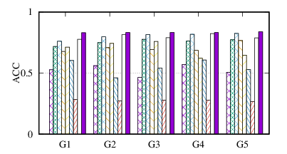
(a)
ACC
on
BrainNet
|
(b)
ACC
on
20news
|
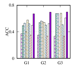
(c)
ACC
on
DBLP
|
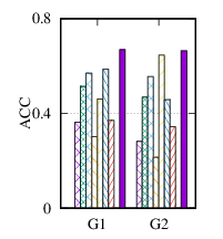
(d)
ACC
on
Flickr
|
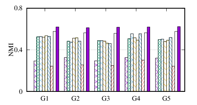
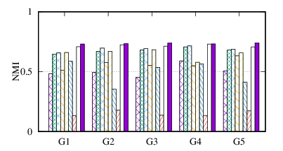
(e)
NMI
on
BrainNet
|
(f)
NMI
on
20news
|
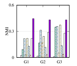
(g)
NMI
on
DBLP
|
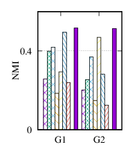
(h)
NMI
on
Flickr
|
 |
Environmental Settings. For all of the embedding methods, we follow [21] to set the dimensionality of node embedding to 100. For other hyperparameters of the baseline methods, we follow the instructions in their papers to search for the optimal values and report the best results. Specifically, for Deepwalk, node2vec, and comE, we set walks per node 𝑟= 10, walk length 𝑙= 80, context size 𝑘= 10, negative samples per node 𝑚= 5. As suggested by [6], we use a grid search over 𝑝,𝑞∈{0.25,0.5,1,2,4} for node2vec. For GraphSAGE, we use its unsupervised loss and feature-less version for a fair comparison. The learning rate is set to 0.01 and the number of maximum iterations is set to 2000. The number of neighbors is 3 for each layer. Negative sampling size is set to 20. For MCA, its model parameter α and η are set to 0.1. For MANE, its model parameter α is set to 0.1. For DMNE, we set 𝑐= 0.98, 𝐾= 3, α= 1 and β= 1. The autoencoder configuration is 𝐵-200 -100 -200 -𝐵. For our method DMGC, the autoencoder configuration is 𝑛𝑖-1024 -100 -1024 -𝑛𝑖 for BrainNet, and 𝑛𝑖-128 -100 -128 -𝑛𝑖 for other datasets. The model parameters α and β are set to 1. A study about these model parameters will be discussed in Sec. 5.5. Our algorithm is implemented with tensorflow 1.12. The learning rate is set to 0.001 and maximum iteration is set to 2000. The dimensionality of cluster centroids in the unified space is set to 20.
(a)
Spectral
|
(b)
Deepwalk
|
(c)
node2vec
|
(d)
GraphSAGE
|
(e)
comE
|
(f)
MANE
|
(g)
DMNE
|
(h)
DMGC
|
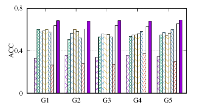
From the figures, we have several observations. First, we can see that our method achieves the best results on all datasets in terms of both metrics. The reason is that DMGC can incorporate complementary information in multi-graph to refine the clustering results. In the meantime, the deep neural network used in DMGC can capture the highly non-linear patterns of nodes. Second, single graph clustering (embedding) methods, such as Spectral, Deepwalk, node2vec, GraphSAGE, and comE suffers from the noises and incompleteness in the single graph. In contrast, multi-graph clustering (embedding) methods, such as DMGC, and DMNE can leverage complementary information different graphs to alleviate this problem, which explains why they generally outperform single graph methods. Third, Spectral and MANE, which are based on eigen-decomposition of adjacency matrices, achieve relatively low accuracy results on BrainNet and DBLP. This is because the adjacency matrices have high dimensionalities and are very sparse. The underlying non-linearity patterns harm the effectiveness of these two methods. In many cases, MANE, is outperformed by Spectral, one possible reason is that its shallow model cannot well capture the complex within- and cross-graph connections in a joint manner. Last, the comparison between DMNE and DMGC shows the advantage of joint optimization for end-to-end node clustering and attentive cluster association across different graphs.
Efficiency Evaluation. To evaluate the efficiency of DMGC, we compare the running time of different multi-graph clustering (embedding) methods in Table 3. We repeat each experiment 5 times and present the average running time.
From Table 3, we observe MCA is the most efficient because of its shallow matrix factorization model. MANE is based on the eigendecomposition of adjacency matrices, thus has a high time cost. Compared to DMNE, our method is trained in end-to-end manner, and does not need pretraining, thus is faster. Overall, DMGC runs in reasonable time w.r.t. the baseline approaches, especially considering its intriguing performance as shown in Fig. 4.
| Dataset | MCA | MANE | DMNE | DMGC |
| BrainNet | 5.52 | 170.09 | 71.72 | 66.25 |
| 20news | 44.93 | 333.42 | 363.16 | 84.50 |
| DBLP | 722.29 | 1,280.61 | 11,252.78 | 433.29 |
| Flickr | 1085.38 | 20,200.95 | >12 hours | 4099.25 |
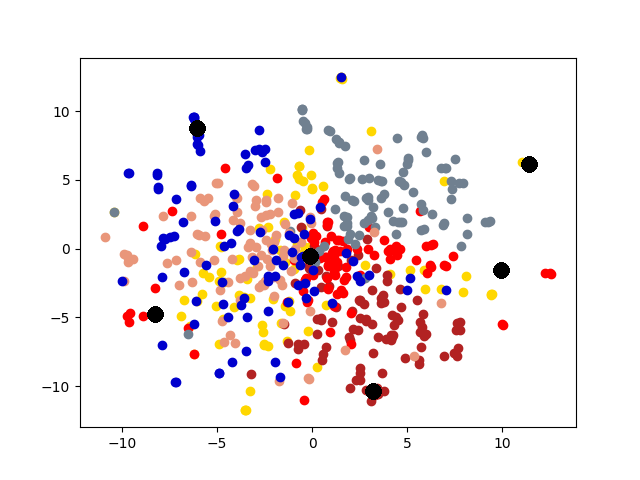
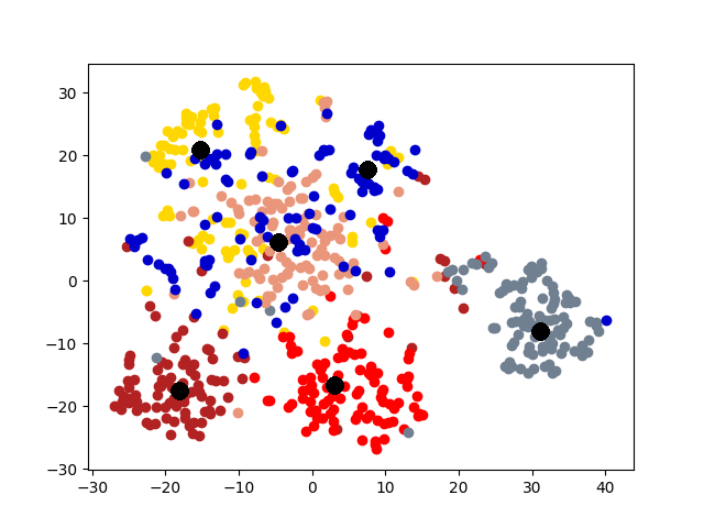
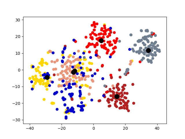
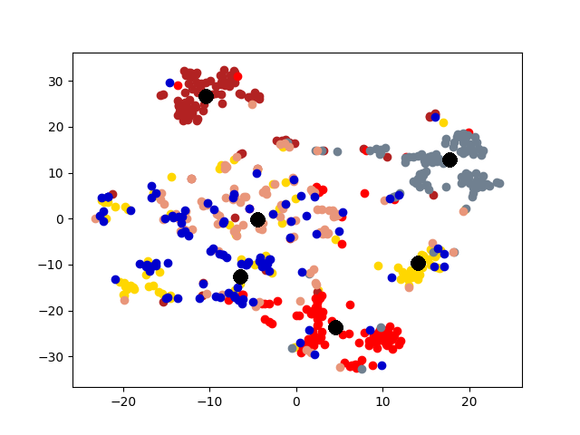
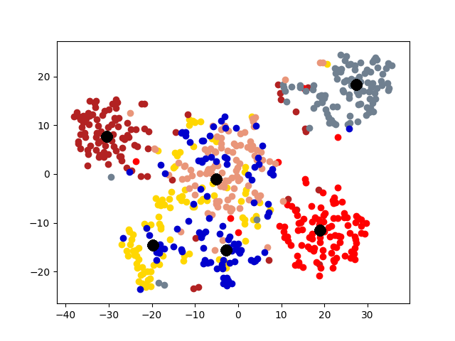
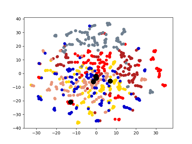
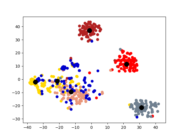
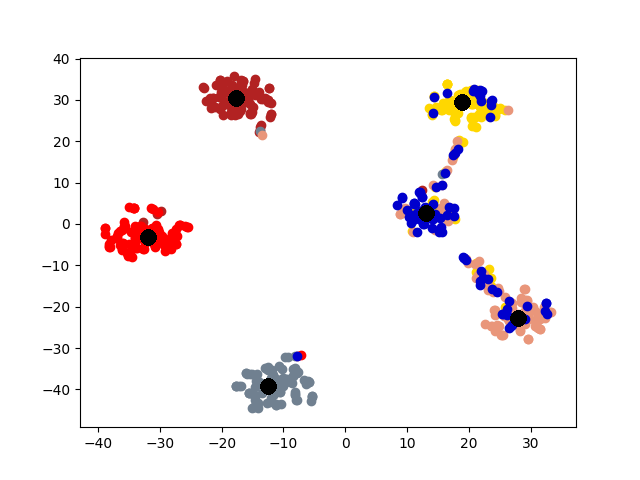
5.4 Visualization. Node Embeddings. To better understand the difference between the compared methods, we use t-SNE [14] to project the node embeddings of each method to a 2D space for visualization. Fig. 5 shows the results on the first graph of 20news dataset, which has 600 nodes. Different colors represent 6 different clusters. The big black dots in the figure represent cluster centroids. From the figure, we can observe that deep models generally outperform shallow models (e.g., Spectral, MANE) in representation learning. Clustering based methods, such as comE and DMGC can detect better community structure with proper centroid positions in the embedding space than single graph embedding methods. Moreover, multi-graph embedding methods DMNE and DMGC can effectively leverage cross-graph relationships to force apart communities. By combining all the above advantages, DMGC obtains the best embedding quality in terms of the community boundary and centroids, which is consistent with the results in Fig. 4.
Cluster Association. Next, we visualize the cross-graph cluster association of DMGC. To this end, we choose the first and second graphs of 20news dataset. For comparison, we select DMNE, another multi-graph embedding method without cluster association. For both methods, the two graphs are embedded to the same hidden space (i.e., the same dimensionality). Fig. 6 shows the comparison. In the figure big yellow and black dots represent cluster centroids in the first and second graphs, respectively. In Fig. 6(b), each community is marked with a label. The prefix “1” and “2” indicate graph ID, the letters, “a”, “b”, etc., indicate cluster ID. Note that clusters with the same ID but in different graphs (e.g., “1a” and “2a”) have more cross-graph relationships than other pairs. As can be seen, DMGC can clearly associate the right cluster pairs by drawing them closely, which facilitates to enlarge community boundaries within each graph for improving clustering accuracy. In contrast, DMNE simply mixes clusters from the two graphs together. When cluster boundary is small (e.g., left bottom of Fig. 6(a)), the associations between clusters are hard to identify.
(a)
DMNE
|
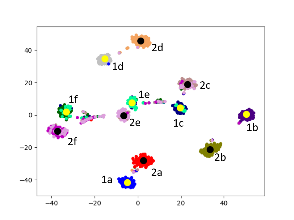
(b)
DMGC
|
5.5 Parameter Sensitivity. In our model in Eq. (14), there are two major parameters α and β. In this section, we evaluate the impacts of them, together with the dimensionality of embedding 𝑑𝑖, on 20news dataset.
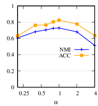
(a)
Parameter
study
of α |
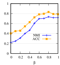
(b)
Parameter
study
of β |
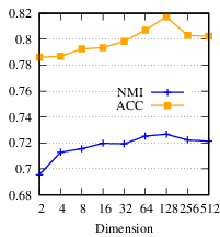
(c)
Parameter
study
of
𝑑𝑖 |
First, we vary α by {0.2, 0.4, 0.6, 0.8, 1, 2, 4}, and fix β= 0.8, 𝑑𝑖= 100. Here, for parameter study purpose, β is set to its optimal value on this dataset instead of the default value 1. Fig. 7(a) shows the ACC and NMI averaged over the five graphs of the 20news dataset. From the figure, our method is quite stable in a wide range of α and achieves the best performance when α= 1 in terms of both ACC and NMI.
Next, we vary β from 0 to 1 by step 0.1, and fix α= 1, 𝑑𝑖= 100. Fig. 7(b) shows the clustering accuracy w.r.t. different β’s. When β= 0, DMGC degrades to single graph clustering without using cross-graph relationships. By comparing the performance at β= 0 and β= 0.8, it is clear DMGC can effectively leverage cross-graph relationships to improve clustering accuracy. Also, the near optimal performance at β= 1 justifies our parameter setting.
To evaluate 𝑑𝑖, we set 𝑑1 = ...= 𝑑𝑔= 𝑑* and vary 𝑑* from 2 to 512, and fix α= 1, β= 0.8. The result is shown in Fig. 7(c). From the figure, DMGC is robust to 𝑑𝑖. Specifically, when 𝑑𝑖 is small, the accuracy increases as 𝑑𝑖 increases because higher dimensionality can encode more useful information. When 𝑑𝑖 reaches its optimal value, the accuracy begins to drop slightly. This is because a too high dimensionality may introduce redundant and noisy information that can harm the clustering performance.
Overall, the performance of DMGC is stable w.r.t. the hyperparameters. The non-zero choices of α and β also justify the importance the proximity constraint and the cross-graph cluster association loss of DMGC in Eq. (14).
To tackle the complex relationships in multi-graph, in this paper, we proposed DMGC for multi-graph clustering. DMGC learns node embeddings in a cluster-friendly space. A novel minimum-entropy based strategy has been proposed to cluster nodes in such a space. Also, we designed an attentive mechanism to capture the cluster-level associations across different graphs to refine the clustering quality. Through extensive experiments on a variety of real-life datasets, we have demonstrated that the proposed DMGC is both effective and efficient.
ACKNOWLEDGMENTS This project was partially supported by NSF projects IIS-1707548 and CBET-1638320.
[1] Sandro Cavallari, Vincent W Zheng, Hongyun Cai, Kevin Chen-Chuan Chang, and Erik Cambria. 2017. Learning community embedding with community detection and node embedding on graphs. In CIKM.
[2] Wei Cheng, Xiang Zhang, Zhishan Guo, Yubao Wu, Patrick F Sullivan, and Wei Wang. 2013. Flexible and robust co-regularized multi-domain graph clustering. In SIGKDD.
[3] Gary William Flake, Robert E Tarjan, and Kostas Tsioutsiouliklis. 2004. Graph clustering and minimum cut trees. Internet Mathematics (2004).
[4] Mahsa Ghorbani, Mahdieh Soleymani Baghshah, and Hamid R. Rabiee. 2018. Multi-layered Graph Embedding with Graph Convolutional Networks. arXiv preprint arXiv:1811.08800 (2018).
[5] Xavier Glorot and Yoshua Bengio. 2010. Understanding the difficulty of training deep feedforward neural networks. In AISTATS.
[6] Aditya Grover and Jure Leskovec. 2016. node2vec: Scalable feature learning for networks. In SIGKDD.
[7] Will Hamilton, Zhitao Ying, and Jure Leskovec. 2017. Inductive representation learning on large graphs. In NeurIPS.
[8] Diederik P Kingma and Jimmy Ba. 2014. Adam: A method for stochastic optimization. arXiv preprint arXiv:1412.6980 (2014).
[9] Thomas N Kipf and Max Welling. 2016. Semi-supervised classification with graph convolutional networks. arXiv preprint arXiv:1609.02907 (2016).
[10] Ru Kong, Jingwei Li, Csaba Orban, Mert Rory Sabuncu, Hesheng Liu, Alexander Schaefer, Nanbo Sun, Xi-Nian Zuo, Avram J Holmes, Simon B Eickhoff, et al. 2018. Spatial topography of individual-specific cortical networks predicts human cognition, personality, and emotion. Cerebral Cortex (2018).
[11] Da Kuang, Chris Ding, and Haesun Park. 2012. Symmetric nonnegative matrix factorization for graph clustering. In SDM. SIAM, 106–117.
[12] Jundong Li, Chen Chen, Hanghang Tong, and Huan Liu. 2018. Multi-Layered Network Embedding. In SDM.
[13] Rui Liu, Wei Cheng, Hanghang Tong, Wei Wang, and Xiang Zhang. 2015. Robust multi-network clustering via joint cross-domain cluster alignment. In ICDM.
[14] Laurens van der Maaten and Geoffrey Hinton. 2008. Visualizing data using t-SNE. JMLR (2008).
[15] Christopher Manning, Prabhakar Raghavan, and Hinrich Schütze. 2010. Introduction to information retrieval. Natural Language Engineering 16, 1 (2010), 100–103.
[16] Nina Mrzelj and Pavlin Gregor Poličar. 2017. Data clustering using stochastic block models. arXiv preprint arXiv:1707.07494 (2017).
[17] Maria CV Nascimento and Andre CPLF De Carvalho. 2011. Spectral methods for graph clustering–a survey. European Journal of Operational Research (2011).
[18] Mark EJ Newman. 2006. Finding community structure in networks using the eigenvectors of matrices. Physical review E (2006).
[19] Jingchao Ni, Shiyu Chang, Xiao Liu, Wei Cheng, Haifeng Chen, Dongkuan Xu, and Xiang Zhang. 2018. Co-regularized deep multi-network embedding. In WWW.
[20] Le Ou-Yang, Hong Yan, and Xiao-Fei Zhang. 2017. A multi-network clustering method for detecting protein complexes from multiple heterogeneous networks. BMC bioinformatics (2017).
[21] Bryan Perozzi, Rami Al-Rfou, and Steven Skiena. 2014. Deepwalk: Online learning of social representations. In SIGKDD. ACM, 701–710.
[22] Benedek Rozemberczki, Ryan Davies, Rik Sarkar, and Charles A. Sutton. 2018. GEMSEC: Graph Embedding with Self Clustering. arXiv preprint arXiv:1802.03997 (2018).
[23] Claude Elwood Shannon. 1948. A mathematical theory of communication. Bell system technical journal (1948).
[24] Jie Tang, Jing Zhang, Limin Yao, Juanzi Li, Li Zhang, and Zhong Su. 2008. Arnetminer: extraction and mining of academic social networks. In SIGKDD.
[25] Wei Tang, Zhengdong Lu, and Inderjit S Dhillon. 2009. Clustering with multiple graphs. In ICDM.
[26] Fei Tian, Bin Gao, Qing Cui, Enhong Chen, and Tie-Yan Liu. 2014. Learning deep representations for graph clustering. In AAAI.
[27] David C Van Essen, Stephen M Smith, Deanna M Barch, Timothy EJ Behrens, Essa Yacoub, Kamil Ugurbil, Wu-Minn HCP Consortium, et al. 2013. The WU-Minn human connectome project: an overview. Neuroimage (2013).
[28] Petar Veličković, Guillem Cucurull, Arantxa Casanova, Adriana Romero, Pietro Lio, and Yoshua Bengio. 2017. Graph attention networks. arXiv preprint arXiv:1710.10903 (2017).
[29] Ulrike Von Luxburg. 2007. A tutorial on spectral clustering. Statistics and computing (2007).
[30] Chi-Jen Wang, Seokjoo Chae, Leonid A Bunimovich, and Benjamin Z Webb. 2017. Uncovering Hierarchical Structure in Social Networks using Isospectral Reductions. arXiv preprint arXiv:1801.03385 (2017).
[31] Daixin Wang, Peng Cui, and Wenwu Zhu. 2016. Structural deep network embedding. In SIGKDD.
[32] Jim Jing-Yan Wang, Halima Bensmail, and Xin Gao. 2012. Multiple graph regularized protein domain ranking. BMC bioinformatics (2012).
[33] Weiran Wang, Raman Arora, Karen Livescu, and Jeff A Bilmes. 2015. Unsupervised learning of acoustic features via deep canonical correlation analysis. In ICASSP.
[34] Xiao Wang, Peng Cui, Jing Wang, Jian Pei, Wenwu Zhu, and Shiqiang Yang. 2017. Community preserving network embedding. In AAAI.
[35] Xufei Wang, Lei Tang, Huan Liu, and Lei Wang. 2013. Learning with multi-resolution overlapping communities. Knowledge and information systems (2013).
[36] Junyuan Xie, Ross Girshick, and Ali Farhadi. 2016. Unsupervised deep embedding for clustering analysis. In ICML.
[37] Carl Yang, Hanqing Lu, and Kevin Chen-Chuan Chang. 2017. Cone: Community oriented network embedding. arXiv preprint arXiv:1709.01554 (2017).


![[ ]
𝐿𝑐 =∑︁ - ∑︁ logσ(q(𝑥𝑖)(q(𝑥𝑖))𝑇)+KL(p(𝑖)||u(𝑖))
𝑖 𝑥](WSDM-sigconf8x.svg)


![(𝑖) ( (𝑖)[(𝑖) ∑︁ (𝑖1)(1) ∑︁ (𝑖𝑔) (𝑔)])
𝝁𝑘 = ReLU W z𝑘 ; 𝑐𝑘𝑙 z𝑙 ;...; 𝑐𝑘𝑙 z𝑙
𝑙 𝑙](WSDM-sigconf15x.svg)