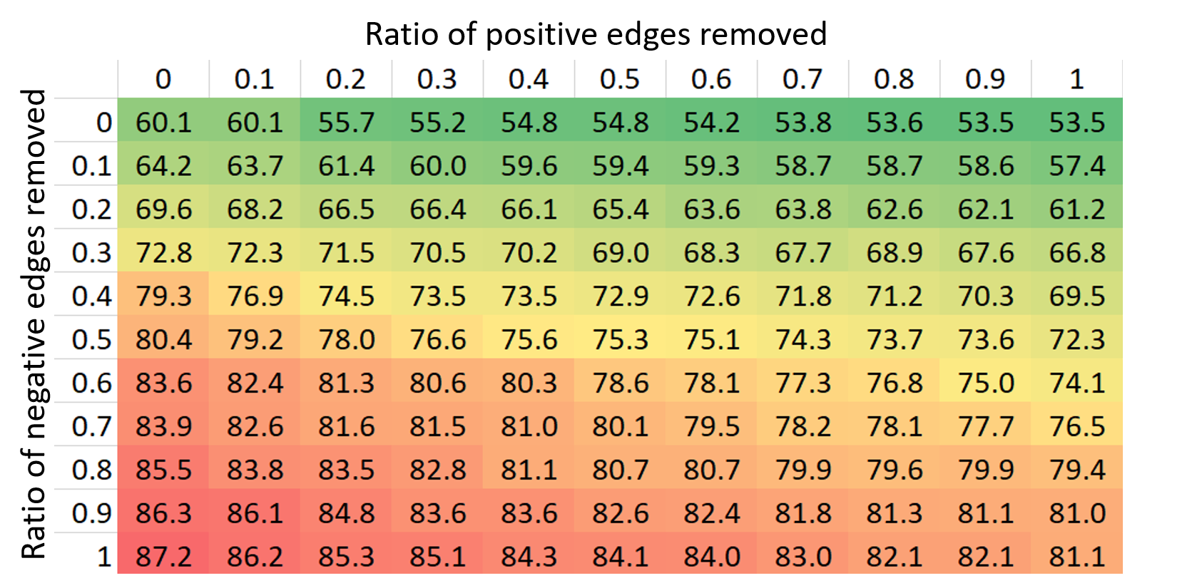
Figure 1: Performance of GCN w.r.t. removing positive and
negative edges on Cora.
Learning to Drop: Robust Graph Neural Network via Topological Denoising
Dongsheng Luo1*, Wei Cheng2*, Wenchao Yu2, Bo Zong2, Jingchao Ni2,
Haifeng Chen2, Xiang Zhang1
1Pennsylvania State University, 2NEC Labs America {dul262,xzz89}@psu.edu,{weicheng,wyu,bzong,jni,haifeng}@nec-labs.com
AbstractGraph Neural Networks (GNNs) have shown to be powerful tools for graph analytics. The key idea is to recursively propagate and aggregate information along edges of the given graph. Despite their success, however, the existing GNNs are usually sensitive to the quality of the input graph. Real-world graphs are often noisy and contain task-irrelevant edges, which may lead to suboptimal generalization performance in the learned GNN models. In this paper, we propose PTDNet, a parameterized topological denoising network, to improve the robustness and generalization performance of GNNs by learning to drop task-irrelevant edges. PTDNet prunes task-irrelevant edges by penalizing the number of edges in the sparsified graph with parameterized networks. To take into consideration of the topology of the entire graph, the nuclear norm regularization is applied to impose the low-rank constraint on the resulting sparsified graph for better generalization. PTDNet can be used as a key component in GNN models to improve their performances on various tasks, such as node classification and link prediction. Experimental studies on both synthetic and benchmark datasets show that PTDNet can improve the performance of GNNs significantly and the performance gain becomes larger for more noisy datasets.
ACM Reference Format:
Dongsheng Luo1*, Wei Cheng2*, Wenchao Yu2, Bo Zong2, Jingchao Ni2, and Haifeng Chen2, Xiang Zhang1. 2021. Learning to Drop: Robust Graph Neural Network via Topological Denoising. In WSDM ’21:International Conference on Web Search and Data Mining, March 08–12, 2021, Jerusalem, Israel .
In recent years, we have witnessed a dramatic increase in our ability to extract and collect data from the physical world. In many applications, data with complex structures are connected for their interactions and are naturally represented as graphs [35, 42, 44]. Graphs are powerful data representations but are challenging to work with because they require modeling both node feature information as well as rich relational information among nodes [5, 17, 40, 51]. To tackle this challenge, various Graph Neural Networks (GNNs) have been proposed to aggregate information from both graph topology and node features [17, 25, 43, 49, 53]. GNNs model node features as messages and propagate them along the edges of the input graph. During the process, GNNs compute the representation vector of a node by recursively aggregating and transforming representation vectors of its neighboring nodes. Such methods have achieved state-of-the-art performances in various tasks, including node classification and link prediction [54, 57].
Despite their success, GNNs are vulnerable to the quality of the given graph due to its recursively aggregating schema. It is natural to ask: is it necessary to aggregate all neighboring nodes? If not, is there a principled way to select which neighboring nodes are not needed to be included? In many real-world applications, graph data exhibit complex topology patterns. Recent works [38, 55] have shown that GNNs are greatly over-smoothed as edges can be pruned without loss of accuracy. Besides, GNNs are easily aggregating task-irrelevant information, leading to over-fitting which weakens the generalization ability. Specifically, from the local perspective, a node might be linked to nodes with task-specific “noisy” edges. Aggregating information from these nodes would impair the quality of the node embedding and lead to unwanted prediction in the downstream task. From the global view, nodes located at the boundary of clusters are connected to nodes from multiple communities. Overwhelming information collected from their neighbors would dilute the true underlying patterns.
As a motivating example, we consider a benchmark dataset Cora [40]. We denote the edges connecting nodes with the same label as positive edges, otherwise, as negative edges. Table 1 shows the statistics of different edges. It is reasonable to consider that passing messages through positive edges leads to high quality node representation, while information aggregated along negative edges impair the performance of GNNs [19]. We adopt Graph Convolutional Network(GCN) [25], a representative GNN, as an example to verify this intuition. We randomly delete some positive and negative edges and conduct GCN on the resulting graphs. As shown in Fig. 1, the performance of GCN increases with more negative edges removed.
| Dataset | # Nodes | # Edges | # Pos. Edges | # Neg. Edges |
| Cora | 2,708 | 5,429 | 4,418 | 1,011 |
Topological denoising is a promising solution to address the above-mentioned challenge by removing “noisy” edges [11, 45]. By denoising the input graph, we can prune away task-irrelevant edges to avoid aggregating unnecessary information in GNNs. Besides, it can also help improve the robustness and alleviate the over-smoothing problem inherent of GNNs [38]. The idea of topological denoising is not new. In fact, this line of thinking has motivated GAT [43] that aggregates neighboring nodes with weights from attention mechanism and thus to some extent alleviate the problem. Other existing methods aim to extract smaller subgraphs from the given graphs to preserve pre-defined properties or randomly remove/sample edges during the training process to prevent GNNs from over-smoothing [17, 38, 41, 46]. However, within unsupervised settings, subgraphs sampled from these approaches may be suboptimal for downstream tasks and also lack persuasive rationales to explain the outcomes of the model for the task. Instead, the task-irrelevant “noisy” edges should be specific to the downstream objective. Besides, in real-life graphs, node contents and graph topology provide complementary information to each other. Denoising process should take both information into consideration, which is overlooked by existing methods.
In this paper, we propose a Parameterized Topological Denoising network (PTDNet) to enhance the performance of GNNs. We use deep neural networks, considering both structural and content information as inputs, to learn to drop task-irrelevant edges in a data-driven way. PTDNet prunes the graph edges by penalizing the number of edges in the sparsified graph with parameterized networks [29, 50]. The denoised graphs are then fed into GNNs for robust learning. The introduced sparsity in the neighboring nodes aggregation has a variety of merits: 1) a sparse aggregation is less complicated and hence generalizes well [15]; 2) it can facilitate interpretability and help infer task-relevant neighbors. Considering the combinatorial nature of the denoising process, we relax the discrete constraint with continuous distributions that could be optimized efficiently with backpropagation, enabling PTDNet to be compatible with various GNNs in both transductive and inductive settings, including GCN [25], Graph Attention Network [43], GraphSage [17], etc. In PTDNet, the denoising networks and GNN are jointly optimized in an end-to-end fashion. Different from conventional methods that remove edges randomly or based on pre-defined rules, the denoising process of PTDNet is guided by the supervision of the downstream objective in the training phase.
To further concern the global topology, the nuclear norm regularization is applied to impose low-rank constraint on the resulting sparsified graph for better generalization. Due to the discontinuous nature of the rank minimization problem, PTDNet smooths the constraint with the nuclear norm, which is the tightest convex envelope of the rank [37]. This regularization denoises the input graph from the global topology perspective by removing edges connecting multiple communities to improve generalization ability and robustness of GNNs [11]. Experimental results on both synthetic and benchmark datasets demonstrate that PTDNet can effectively enhance the performance and robustness of GNNs.
GNNs are powerful tools to investigate the graph data with node contents. GNN models utilize the message passing mechanism to encode both graph structural information and node features into vector representations. These vectors are then used to node-level or graph-level downstream tasks. GNNs were initially proposed in [16], and extended in [39]. These methods learn node representations by iteratively aggregating neighbor information until reaching a static state. Inspired by the success of convolutional neural networks (CNNs) in computer vision, graph convolutional networks in the graph spectral domain were proposed based upon graph Fourier transform [4]. Multiple extensions were further proposed [9, 25, 28, 31, 39, 43]. The express power of GNNs were analyzed in [49]. DropEdge and PairNorm investigated the over-smoothing problem of stacking multiple GNN layers [38, 55].
Graph Sparsification and Sampling. Conventional graph sparsification approximates the large input graph with a sparse subgraph to enable efficient computation, and at the same time preserve certain properties. Different notions have been extensively studied including pairwise distances betweenness [7], sizes of all cuts [2], node degree distributions [10], and spectral properties [1, 18]. These methods remove edges only based upon the structural information, which limits their power when combining with GNNs. Besides, without supervised feedback from the downstream task, these approaches may generate subgraphs with suboptimal structural properties. NeuralSparse [56] learns 𝑘-neighbor subgraphs for robust graph representation learning by selecting at most 𝑘 edges for each nodes. The 𝑘-neighbor assumption however limits its learning power and may lead to suboptimal performance in generalization.
Recently, graph sampling has been investigated in GNNs for fast computation and better generalization capacity, including neighbor-level [17], node-level [6, 20, 52], and edge-level sampling methods [38]. Unlike these methods that randomly sample edges in the training phase, PTDNet utilizes parametrized networks to actively remove task-specific noisy edges. With supervised guidance from downstream objective, the generated subgraphs benefit GNNs in not only robustness but also accuracy and interpretability. Besides, PTDNet has better generalization capacity as the parametrized networks can be used for inductive inference.
Notations. In general, we use lowercase, bold uppercase, and bold lowercase letters for scalars, matrices, and vectors, respectively. For example, we use Z to denote a matrix, whose 𝑖,𝑗-th entry is denoted by 𝑧𝑖𝑗 , a lowercase character with subscripts. Let 𝐺= (V,E) represent the input graph with 𝑛 nodes, where V,E stand for its node/edge set, respectively. The adjacency matrix of 𝐺 is denoted by A ∈R𝑛×𝑛 . Node features are denoted by matrix X ∈R𝑛×𝑚 with 𝑚 as the dimensionality of node features. We use Y to denote the labels in the downstream task. For instance, in the node classification task, Y ∈R𝑛×𝑐 represents node labels, where 𝑐 is the number of classes.
GNN layer. Applying a GNN layer consists of the propagation step and the output step [57]. At the propagation step, the aggregator first computes the message for each edge. For an edge (𝑣𝑖 ,𝑣𝑗 ), the aggregator takes the representations of 𝑣𝑖 and 𝑣𝑗 in previous layer as inputs, denoted by h𝑖 𝑡-1, and h𝑗 𝑡-1, respectively. Then, the aggregator collects messages from local neighborhoods for each node 𝑣𝑖 . At the output step, the updater computes its new hidden representation, denoted by h𝑣 𝑡 .
GNN models adopt message passing mechanisms to propagate and aggregate information along the input graph to learn node representations. The performances can be heavily affected by the quality of the input graph. Messages aggregated along “noisy” edges may decrease the quality of node embeddings. Overwhelming information from multiple communities put GNNs at the risk of over-smoothing, especially when multiple GNN layers are stacked [30, 38, 55]. Existing methods either utilize graph sparsification strategies to extract subgraphs or randomly sample graphs to enhance the robustness of GNNs. Basically, they are conducted in an unsupervised way, limiting their ability to filter out task-specific noisy edges.
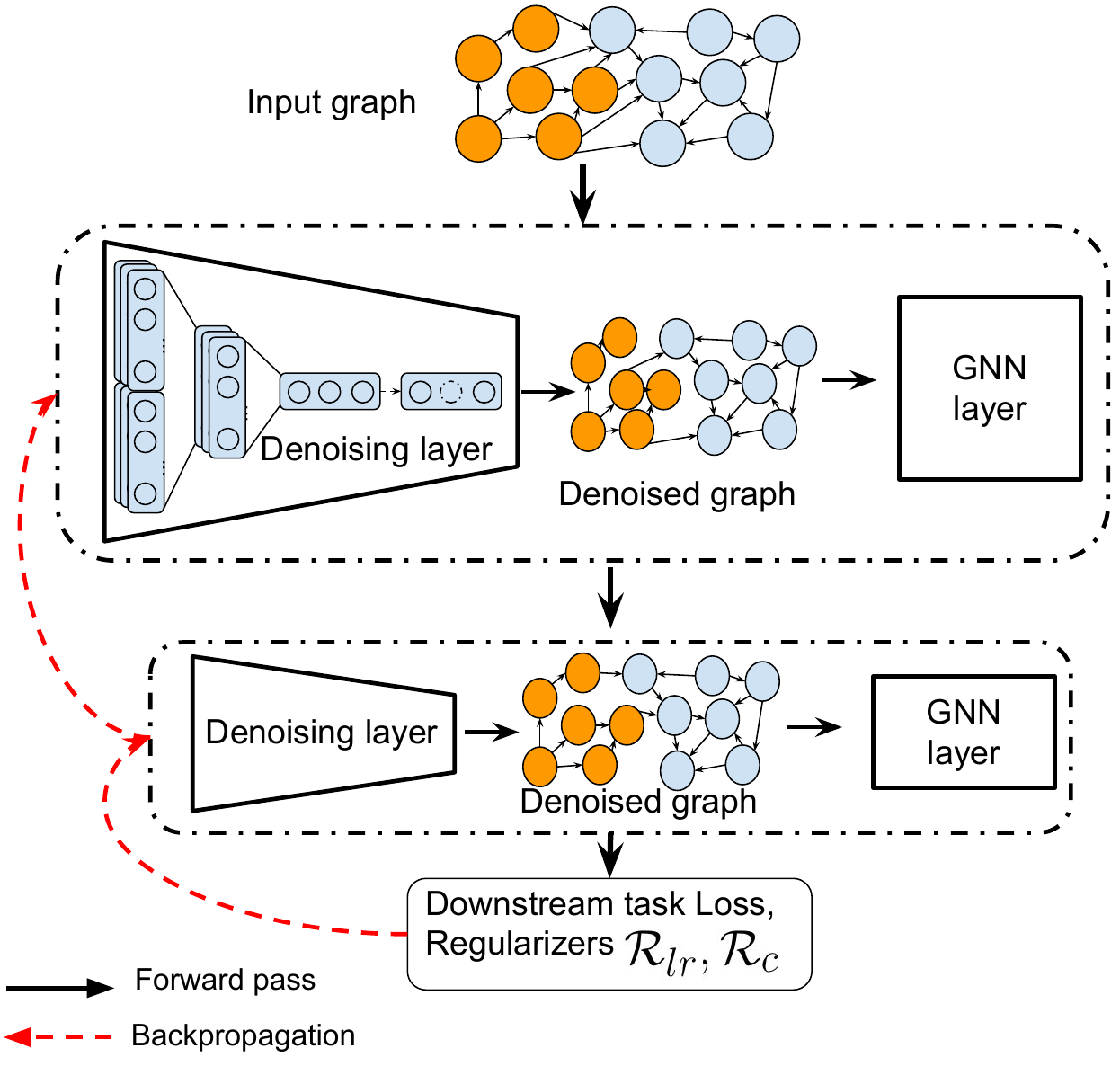
The core idea of PTDNet is to actively filter out task-specific noisy edges in the input graph with a parameterized network. It consists of the denoising network and general GNNs. GNNs can be applied under both inductive and transductive settings. We first give an overview of PTDNet in Sec. ??, followed by details of the denoising network in Sec. 4.2. To enhance the generalization ability of PTDNet, we further introduce the low-rank constraint on resulting graphs and provide smoothing relaxation to achieve an end-to-end model.
4.1 The overall architecture. The architecture of PTDNet is shown in Fig. 2(a). It consists of two major components, the denoising networks and the GNNs. The denoising network is a multi-layer network that samples a subgraph from a learned distribution of edges. PTDNet is compatible with most existing GNNs, such as GCN [25], GraphSage [17], GAT [43], GIN [49], etc. With relaxations, the denoising network is differentiable and can be jointly optimized with GNNs guided by supervised downstream signals.
4.2.1 Graph edge sparsification. The goal of the denoising network is to generate a subgraph filtering out task-irrelevant edges for GNN layers. For the 𝑙-th GNN layer, we introduce a binary matrix Z𝑙 ∈{0,1}|V|×|V|, with 𝑧𝑢,𝑣 𝑙 denoting whether the edge between node 𝑢 and 𝑣 is present (0 indicates noisy edge). Formally, the adjacency matrix of the resulting subgraph is A𝑙 = A ⊙Z𝑙 ,where ⊙ is the element-wise product. One way to reduce noisy edges with the least assumptions about A𝑙 is to directly penalize the number of non-zero entries in Z𝑙 of different layers.
| (1) |
where I[·] is an indicator function, with I[𝑇𝑟𝑢𝑒]= 1 and I[𝐹𝑎𝑙𝑠𝑒]= 0, ||·||0 is the ℓ0 norm. There are 2|E| possible states of Z𝑙 . Because of its nondifferentiability and combinatorial nature, optimizing this penalty is computationally intractable. Therefore, we consider each binary number 𝑧𝑢,𝑣 𝑙 to be drawn from a Bernoulli distribution parameterized by π𝑢,𝑣 𝑙 , i.e., 𝑧𝑢,𝑣 𝑙 ~𝐵𝑒𝑟𝑛(π𝑢,𝑣 𝑙 ). The matrix of π𝑢,𝑣 𝑙 ’s is denoted by Π𝑙 . Then, penalizing the non-zero entries in Z𝑙 , i.e., the number of edges being used, can be reformulated as regularizing ∑ (𝑢,𝑣)∈Eπ𝑢,𝑣 𝑙 [29].
Since π𝑢,𝑣 𝑙 is optimized jointly with the downstream task, it
describes the task-specific quality of the edge (𝑢,𝑣). A small value of
π𝑢,𝑣 𝑙 indicates the edge (𝑢,𝑣) is more likely to be noise and should be
with small weight or even be removed in the following GNN. Although
the regularization of the reformulated form is continuous, the
adjacency matrix of the resulting graph is still generated by a binary
matrix Z𝑙 . The expected cost of downstream task could be modeled as
𝐿({Π𝑙 }𝑙=1𝐿 )= EZ1~𝑝(Π1), ,Z𝐿 ~𝑝(Π𝐿 )𝑓({Z𝑙 }𝑙=1𝐿 ,X). To minimize
the expected cost via gradient descent, we need to estimate the
gradient ∇Π𝑙 EZ1~𝑝(Π1),
,Z𝐿 ~𝑝(Π𝐿 )𝑓({Z𝑙 }𝑙=1𝐿 ,X). To minimize
the expected cost via gradient descent, we need to estimate the
gradient ∇Π𝑙 EZ1~𝑝(Π1), ,Z𝐿 ~𝑝(Π𝐿 )𝑓({Z𝑙 }𝑙=1𝐿 ,X), 𝑙∈[1,2,
 ,𝐿].
Existing methods adopt various estimators to approximate the
gradient, including score function [48], straight-through [3], etc.
However, these methods suffer from either high variance or biased
gradients [33]. In addition, to make PTDNet suitable for the inductive
setting and enhance generalization ability, a parameterized method for
modeling Z𝑙 should be adopted.
,𝐿].
Existing methods adopt various estimators to approximate the
gradient, including score function [48], straight-through [3], etc.
However, these methods suffer from either high variance or biased
gradients [33]. In addition, to make PTDNet suitable for the inductive
setting and enhance generalization ability, a parameterized method for
modeling Z𝑙 should be adopted.
4.2.2 Continuous relaxation with parameterized networks. To efficiently optimize subgraphs with gradient methods, we adopt the reparameterization trick [22] and relax the binary entries 𝑧𝑢,𝑣 𝑙 from being drawn from a Bernoulli distribution to a deterministic function 𝑔 of parameters α𝑢,𝑣 𝑙 ∈R and an independent random variable ϵ𝑙 . That is 𝑧𝑢,𝑣 𝑙 = 𝑔(α𝑢,𝑣 𝑙 ,ϵ𝑙 ).
| (2) |
To enable the inductive setting, we should not only figure out which edges but also why they should be filtered out. To learn to drop, for each edge (𝑢,𝑣), we adopt parameterized networks to model the relationship between the task-specific quality π𝑢,𝑣 𝑙 and the node information including node contents and topological structure. In the training phase, we jointly optimize denoising networks and GNNs. In the testing phase, the input graphs could also be denoised with the learned denoising networks. Since we need to compute a subgraph of the input graph, the time complexity of the denoising network in the inference phase is linear to the number of edges 𝑂(|E|).
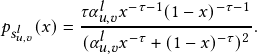
Following [43], we adopt deep neural networks to learn the parameter α𝑢,𝑣 𝑙 that controls whether to remove the edge (𝑢,𝑣). Without loss of generality, we focus on a node 𝑢 in the training graph. Let N𝑢 be its neighbors. For the 𝑙-th GNN layer, we calculate α𝑢,𝑣 𝑙 for node 𝑢 and 𝑣∈N𝑢 with α𝑢𝑣 𝑙 = 𝑓θ𝑙 𝑙 (h𝑢 𝑙 ,h𝑣 𝑙 ), where 𝑓θ𝑙 𝑙 is an MLP parameterized by θ𝑙 . To get 𝑧𝑢,𝑣 𝑙 , we utilize the concrete distribution along with hard sigmoid function [29, 32]. First, we draw 𝑠𝑢,𝑣 𝑙 from a binary concrete distribution with α𝑢𝑣 𝑙 parameterizing the location [22, 32]. Formally,
| (3) |
where τ∈R+ indicates the temperature and σ(𝑥)=  is the
sigmoid function. With τ>0, the function is smoothed with a
well-defined gradient
is the
sigmoid function. With τ>0, the function is smoothed with a
well-defined gradient  , enabling efficient optimization of the
parameterized denoising network.
, enabling efficient optimization of the
parameterized denoising network.
Since the binary concrete distribution has a range of (0,1), to encourage the weights for task-specific noisy edges to be exactly zeros, we first extend the range to (γ,ζ), with γ<0 and ζ>1 [29]. Then, we compute 𝑧𝑢,𝑣 𝑙 by clipping the negative values to 0 and values larger than 1 to 1.
| (4) |
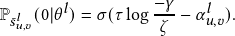
Within the above formulation, the constraint on the number of non-zero entries in Z𝑙 in Eq.( 1) can be reformulated with
| (5) |
P 𝑢,𝑣 𝑙 (0|θ𝑙 ) is the cumulative distribution function (CDF) of 𝑢,𝑣 𝑙 .
As shown in [32], the density of 𝑠𝑢,𝑣 𝑙 is
| (6) |
The CDF of variable 𝑠𝑢,𝑣 𝑙 is
| (7) |
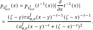
Since the function 𝑢,𝑣 𝑙 = 𝑡(𝑠𝑢,𝑣 𝑙 ) in Eq. (4) is monotonic. The probability density function of 𝑢,𝑣 𝑙 is
| (8) |
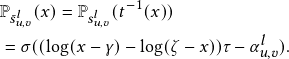
Similarly, we have the CDF of 𝑢,𝑣 𝑙
| (9) |
By setting 𝑥= 0, we have the
| (10) |
Algorithm 1 summarizes the overall training of PTDNet.
 𝑣 |𝑣∈V}←prediction with H𝐿 .
 ,Y)and regularizors.
 𝑙𝑟
𝑙𝑟
 𝑖 𝑙 ←
𝑖 𝑙 ←![√︃---------------
[(v𝑙𝑖)𝑇Bv𝑙𝑖]/[(v𝑙𝑖)𝑇v𝑙𝑖]](main19x.png)
 𝑙𝑟 ←∑
𝑙=1𝐿 ∑𝑖=1𝐾 |
𝑙𝑟 ←∑
𝑙=1𝐿 ∑𝑖=1𝐾 | 𝑖 𝑙 |
2
𝑖 𝑙 |
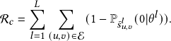
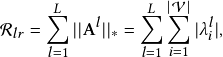
24.3 The low-rank constraint. In the previous section, we introduced parameterized networks to remove the task-specific noisy edges from the local neighborhood perspective. In real-life graph data, nodes from multiple classes can be divided into different clusters. Intuitively, nodes from different topological communities are more likely with different labels [13]. Hence, edges connecting multiple communities are highly possible noise for GNNs. Based upon this intuition, we further introduce a low-rank constraint on the adjacency matrix of the resulting subgraph to enhance the generalization capacity and robustness, since the rank of the adjacency matrix reflects the number of clusters. This regularization denoises the input graph from the global topology perspective by encouraging the denoising networks to remove edges connecting multiple communities such that the resulting subgraphs to have dense connections within communities while sparse between them [24]. Recent work also shows that graphs with low rank are more robust to network attacks [11, 23]. Formally, the straightforward regularizer R𝑙𝑟 for low-rank constraint of PTDNet is ∑ 𝑙=1𝐿 Rank(A𝑙 ), where A𝑙 is the adjacency matrix for the 𝑙-th GNN layer. It has been shown in previous studies that the matrix rank minimization problem (RMP) is NP-hard [8]. We approximately relax the intractable problem with the nuclear norm, which is the convex surrogate for RMP problem [14]. The nuclear norm of a matrix is defined as the sum of its singular values. It is a convex function that can be optimized efficiently. Besides, previous studies have shown that in practice, nuclear norm constraints produce very low-rank solutions [11, 14, 37]. With nuclear norm minimization, the regularizer is
| (11) |
where λ𝑖 𝑙 is the 𝑖-th largest singular values of graph adjacency matrix A𝑙 .
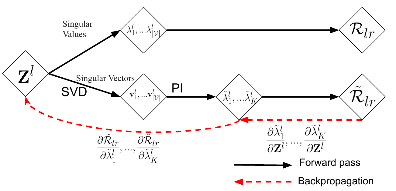
Singular value decomposition (SVD) is required to optimize the nuclear norm regularization. However, SVD may lead to unstable results during backpropagation. As shown in [21], the partial derivatives of the nuclear norm requires computing of a matrix M𝑙 with elements
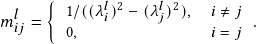
| (12) |
When (λ𝑖 𝑙 )2 -(λ𝑗 𝑙 )2 is small, the partial derivatives become very large, leading to an arithmetic overflow. Besides, the gradient-based optimization on SVD is time-consuming. The Power Iteration (PI) method with deflation procedure is one way to solve this problem [34, 36, 47]. PI approximately computes the largest eigenvalue and the dominant eigenvector of the matrix (A𝑙 )*A𝑙 with an iterative procedure from a randomly initiated vector. (A𝑙 )* stands for the transpose-conjugate matrix of A𝑙 . The largest singular value of A𝑙 is then the square root of the largest eigenvalues. To calculate other eigenvectors, the deflation procedure is involved to iteratively remove the projection of the input matrix on this vector. However, PI may output inaccurate approximations if two eigenvalues are close to each other. The situation becomes worse when we consider eigenvalues near zero. Besides, with randomly initiated vectors, PI may need more iterations to get a precise approximation.
To address the problem, we combine SVD and PI [47] and further
relax the nuclear norm to Ky Fan 𝐾-norm [12], which is the sum of top
𝐾, 1 ≤𝐾≪|V|, largest singular values. Fig. 2(b) shows the forward
pass and backpropagation of the nuclear norm. In the forward pass, as
shown in Algorithm 2, SVD is used to calculate singular values, left
and right singular vectors. Then we get the nuclear norm as the
regularization loss. In order to minimize the nuclear norm, we utilize
the power iteration to compute top 𝐾 singular values, denoted by
 1𝑙 ,...
 𝐾 𝑙 . Note that the PI process does not update the values in
singular vectors and singular values. It only serves to compute
the gradients during backpropagation, which is shown with
red dot lines in Fig. 2(b). We estimate the nuclear norm with
𝐾 𝑙 . Note that the PI process does not update the values in
singular vectors and singular values. It only serves to compute
the gradients during backpropagation, which is shown with
red dot lines in Fig. 2(b). We estimate the nuclear norm with
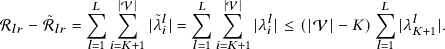
 𝑙𝑟 = ∑
𝑙=1𝐿 ∑𝑖=1𝐾 |
𝑙𝑟 = ∑
𝑙=1𝐿 ∑𝑖=1𝐾 | 𝑖 𝑙 |.
  𝑙𝑟 is a lower bound function of R𝑙𝑟 with
gap
𝑙𝑟 is a lower bound function of R𝑙𝑟 with
gap
| (13) |
It is obvious that ⌈ ⌉
⌉ 𝑙𝑟 is the upper bound of R𝑙𝑟 . We dismiss the
constant coefficient and minimize
𝑙𝑟 is the upper bound of R𝑙𝑟 . We dismiss the
constant coefficient and minimize  𝑙𝑟 as the low-rank constraint.
In this section, we empirically evaluate the robustness and effectiveness of PTDNet with both synthetic and benchmark datasets. First, we apply PTDNet to popular GNN models for node classification on benchmark datasets. Second, we evaluate the robustness of PTDNet by injecting additional noise. Moreover, we also provide insight into the denoising process by checking the edges removed by PTDNet. We also conduct comprehensive experiments to uncover insights of PTDNet, including empirically demonstrating the effects of regularizers, parameter study, analyzing the over-smoothing problem inherent in GNNs, and applying PTDNet to another downstream task, i.e., link prediction.
| Dataset | Cora | Citeseer | Pubmed | PPI |
| Nodes | 2,708 | 3,327 | 19,717 | 56,944 |
| Edge | 5,429 | 4,732 | 44,338 | 818,716 |
| Fea. | 1,433 | 3,703 | 500 | 50 |
| Classes | 7 | 6 | 3 | 121 |
| Train. | 140 | 120 | 100 | 44,906 |
| Val. | 500 | 500 | 500 | 6,514 |
| Test. | 1,000 | 1,000 | 1,000 | 5,524 |
5.1 Experimental setup. Datasets. Four benchmark datasets are adopted in our experiments. Cora, Citeseer, and Pubmed are citation graphs where each node is a document and edges describe the citation relationship. A document is assigned with a unique label based on its topic. Node features are bag-of-words representations of the documents. We follow the standard train/val/test splits in [25, 43] with very scarce labelled nodes, which are different from the full-supervised setting in DropEdge [38]. PPI contains graphs describing protein-protein interaction in different human tissues. Positional gene sets, motif gene sets, and immunological signatures are used as node features. Gene ontology sets are used as labels. The statistics of these datasets are listed in Table 2. Implementations & metrics. We consider three representative GNNs as backbones, including GCN [25], GraphSage [17], GAT [43]. Note that our model is a general framework that is compatible with diverse GNN models. Recent sophisticated models can also be combined with our framework to improve their performances and robustness. Achieving SOTA performances by using a complex architecture is not the main research point of this paper. We compare with most recent state-of-the-art sampling and sparsification methods, DropEdge [38] and NeuralSparse [56]. For GraphSage, we use the mean aggregation. We follow the experimental setting in [38] to perform a random hyper-parameter search for each model. For each setting, we run 10 times and report the average results. Parameters are tuned via cross-validation. We also include a variant of PTDNet by removing the low-rank constraint as the ablation study. For single-label classification datasets, including Cora, Citeseer, and Pubmed, we evaluate the performance with accuracy [25]. For PPI, we evaluate with micro-F1 scores [17].
All experiments are conducted on a Linux machine with 8 NVIDIA Tesla V100 GPUs, each with 32GB memory. CUDA version is 9.0 and Driver Version is 384.183. All methods are implemented with Tensorflow 1.12.
| Backbone | Method | Cora | Citeseer | Pubmed | PPI |
|
GCN | Basic | 0.811 ±0.015 | 0.703 ±0.012 | 0.790 ±0.020 | 0.660 ±0.024 |
| DropEdge | 0.809 ±0.035 | 0.722 ±0.032 | 0.785 ±0.043 | 0.606 ±0.041 | |
| NeuralSparse | 0.821 ±0.014 | 0.715 ±0.014 | 0.788 ±0.018 | 0.651 ±0.014 | |
| PTDNet-wl | 0.824 ±0.018 | 0.717 ±0.170 | 0.791 ±0.012 | 0.752 ±0.017 | |
| PTDNet | 0.828 ±0.026 | 0.727 ±0.018 | 0.798 ±0.024 | 0.803 ±0.008 | |
|
GraghSage | Basic | 0.792 ±0.027 | 0.676 ±0.023 | 0.767 ±0.020 | 0.618 ±0.014 |
| DropEdge | 0.787 ±0.023 | 0.670 ±0.031 | 0.748 ±0.026 | 0.610 ±0.035 | |
| NeuralSparse | 0.793 ±0.021 | 0.674 ±0.011 | 0.751 ±0.021 | 0.626 ±0.023 | |
| PTDNet-wl | 0.794 ±0.026 | 0.678 ±0.022 | 0.770 ±0.024 | 0.645 ±0.020 | |
| PTDNet | 0.803 ±0.019 | 0.679 ±0.018 | 0.771 ±0.010 | 0.648 ±0.025 | |
|
GAT | Basic | 0.830 ±0.007 | 0.721 ±0.009 | 0.790 ±0.008 | 0.973 ±0.012 |
| DropEdge | 0.832 ±0.040 | 0.709 ±0.020 | 0.779 ±0.019 | 0.850 ±0.038 | |
| NeuralSparse | 0.834 ±0.015 | 0.724 ±0.026 | 0.780 ±0.017 | 0.921 ±0.018 | |
| PTDNet-wl | 0.837 ±0.022 | 0.723 ±0.014 | 0.792 ±0.014 | 0.978 ±0.018 | |
| PTDNet | 0.844 ±0.023 | 0.737 ±0.031 | 0.793 ±0.015 | 0.980 ±0.022 | |
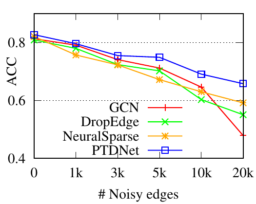
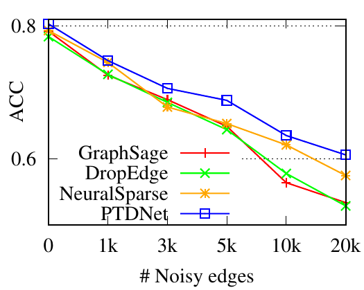
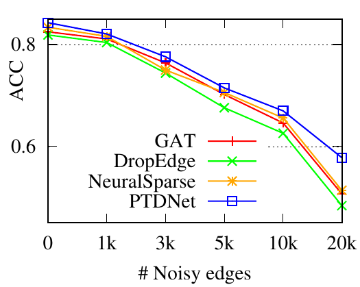
5.3 Robustness evaluation. In this part, we evaluate the robustness of PTDNet by manually including noisy edges. We use the Cora dataset and randomly connect 𝑁 pairs of previously unlinked nodes with 𝑁 ranging from 1000 to 20,000. We compare the proposed method to baselines with all there backbones. Performances are shown in Fig. 3. We have the following observations. 1) PTDNet consistently outperforms DropEdge, NeuralSparse and the basic backbones with various numbers of noisy edges. The comparison demonstrates the robustness of PTDNet. 2) DropEdge randomly samples a subgraph for GNN layers. In most cases, DropEdge reports worse performances than the original backbones. The comparison demonstrates that a random sampling strategy used in DropEdge is vulnerable to noisy edges. 3) NeuralSparse selects noise edges guided by task signals thus achieves better results than basic backbones. However, it selects at most 𝑘 edges for each nodes, which may lead to suboptimal performance. 4) The margins between results of PTDNet and basic backbones become large when more noise are injected. Specifically, PTDNet relatively improves the accuracy scores by 37.37% for GCN, 13.4% for GraphSage, and 16.1% for GAT with 20,000 noisy edges.
5.4 On denoising process. In this section, we use controllable synthetic datasets to analyze the denoising process of PTDNet, which has 5 labels and 30 features per node. We first randomly sample five 30-dimensional vectors as the centroids, one for each label. Then, for each label, we sample nodes from a Gaussian distribution with the centroid as the mean. The variance, which controls the quality of content information is set to 80. The number of nodes for each label is drawn from another Gaussian distribution N(200,25). To validate GNNs on fusing node content and topology, we build a graph containing complementary information with node features. Specifically, we use the distance between a node and the centroid node of its label as the metric to evaluate the quality of the node feature. The probability that it connects to another node with a different label is positively proportional to the feature quality. The resulting graph contains 1,018 nodes and 4,945 edges. We randomly select 60/20/20% nodes for training/validation/testing, respectively.
We use GCN as the backbone for example. The denoising process of the first PTDNet layer is shown in Fig. 4. Red lines represent the mean weight, i.e., 𝑧 in Sec. ??, of positive edges (edges connected nodes with the same label), and blue dotted lines are for negative edges. Fig. 4(a), 4(b) count the edges linked with a training/testing node, respectively. We also show the results of DropEdge to see the case of random selection. These figures demonstrate that DropEdge, an unparameterized method, cannot actively drop the task-irrelevant edges. While PTDNet can detect negative edges and remove or assign them with lower weights. The denoising process of PTDNet leads to higher accuracy with more iterations, which is shown in Fig. 4(c). In addition, the consistent performance of PTDNet on testing nodes shows that our parameterized method can still learn to drop negative edges in the testing phase, demonstrating the generalization capacity of PTDNet. Besides, we plot the degree(volume) distribution of the input graph, subgraph sampled by DropEdge and PTDNet in Fig. 4(d). We observe that both PTDNet and DropEdge can keep the distribution property of the input graph.
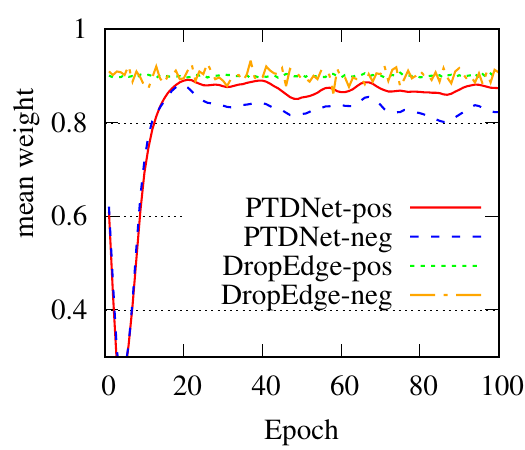
(a)
Training
edges |
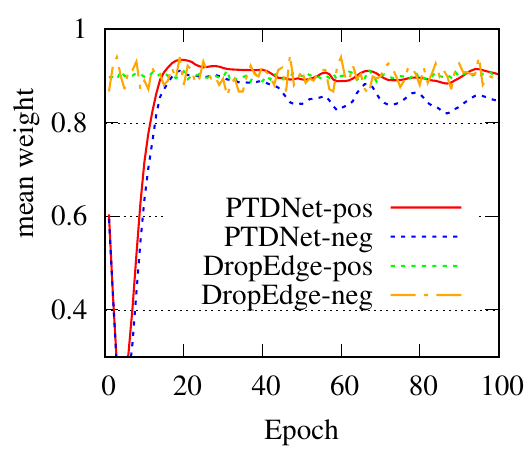
(b)
Testing
edges |
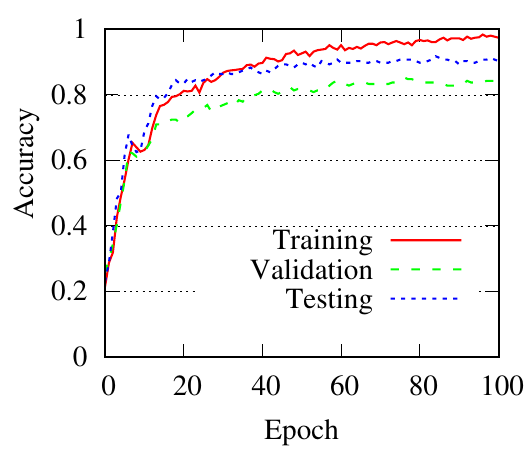
(c)
PTDNet
accuracy |
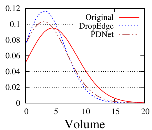
(d)
Degree
distribution |
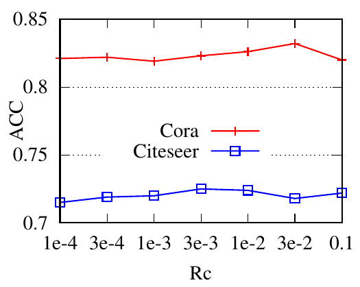
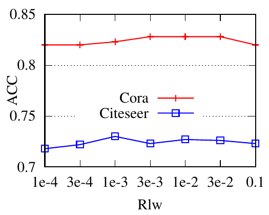
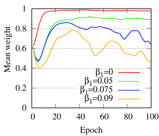
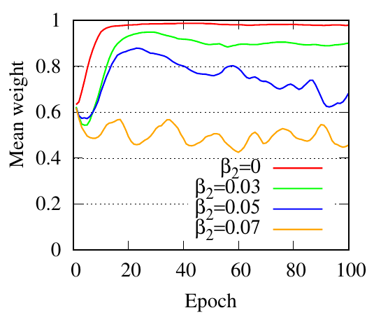
5.5 Effects of regularizers. In this part, we adopt GCN as the backbone to analyze the effects of regularizers. We first show the accuracy performance of PTDNet w.r.t coefficients for regularizers in Fig. 5. For each choice, we fix that value for the coefficient and use the genetic algorithm to search other hyper-parameters. The best performances are reported here. In general, the performance first increases and then drops as coefficients increase. Since the benchmark datasets are relatively clean. To better show the effects of the proposed two regularizers: R𝑐 and R𝑙𝑤 . We synthesize datasets with controllable properties instead. We introduce two hyper-parameters β1 and β2 for regularizers R𝑐 , and R𝑙𝑤 , respectively. These two hyper-parameters affect the ratio of edges to be removed. We first dismiss the low-rank constraint by setting β2 = 0. With different choices of β1 (0, 0.05, 0.075, 0.9), we show mean weights (i.e., 𝑧) of edges during iterations in Fig. 6(a). The figure shows that with a larger hyper-parameter for R𝑐 , PTDNet achieves a more sparse subgraph. Similar observations can be found in Fig. 6(b), where β1 = 0 and only the low-rank constraint is considered.
To demonstrate the effects of including regularizers on the generalization capacity of PTDNet. We synthesize four datasets with various topology properties. The percentages of positive edges in these four datasets range from 0.5 to 0.85. We tune the β1 and β2 separately by setting the other one to 0. The best options of β1 and β2 for these four datasets are shown in Table 4. The table shows that for datasets with poor topological qualities, regularizers should be assigned with higher weights, such that PTDNet can denoise more task-irrelevant edges. On the other hand, for datasets with good structure, i.e., the ratio of positive edges is over 0.85, β1 or β2 should be with relatively small values to keep more edges.
| #pos edge/#all edges | Best β1 | Best β2 |
| 0.85 | 0.01 | 0.05 |
| 0.7 | 0.04 | 0.07 |
| 0.6 | 0.08 | 0.08 |
| 0.5 | 1.0 | 0.1 |
| original |
|
|
|
|||||||
 | 0.211 | 0.206 | 0.189 | 0.190 | ||||||
Low-rank constraint R𝑙𝑤 is introduced to enhance the generalization of PTDNet by setting a constraint on edges connecting nodes from different communities. We use a synthetic dataset to show the influence of R𝑙𝑤 . We adopt the spectral clustering to group nodes into 5 communities. As shown in Table 5, the ratio of cross-community edges is 0.211 in the original graph. We fist adopt PTDNet with β1 = 0.05,β2 = 0 on the dataset. The ratio in the subgraph generated by the first layer is 0.206. By considering low-rank constraint and setting β1 = 0,β2 = 0.05, the ratio drops to 0.189, showing the effectiveness of low-rank constraint on removing cross-community edges.
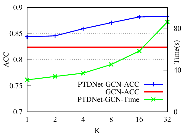
5.6 Impacts of approximate factor 𝐾. In Sec. ??, 𝐾 is the approximate factor in the low-rank constraint. In this part, we the synthetic dataset used in Sec. 5.4. We do not utilize the early stop strategies and fix the number of epochs to 300. We range 𝐾 from 1 to 32 and adopt 2 layer GCN with 256 hidden units as the backbone. The accuracy and running time are shown in Fig. 7. From the figure, we can see that the accuracy performance increase with the larger 𝐾, which is consistent with Eq. 13 that larger 𝐾 indicates tighter bound. At the same time, it leads to more running time. Besides, PTDNet can achieve a relatively high performance even when 𝐾 is small.
5.7 On over-smoothing. The over-smoothing problem exists when multiple GNN layers are stacked [27]. DropEdge alleviates this problem by random drop edges during the training phase. Removing certain edges makes the graph more sparse and reduces messages passing along edges [38]. However, As an unparameterized method, DropEdge is not utilized during the testing phase, which limits its power on preventing the over-smoothing problem, especially on very dense graphs. On the other hand, our PTDNet is a parameterized method, which learns to drop in both training and testing phases.
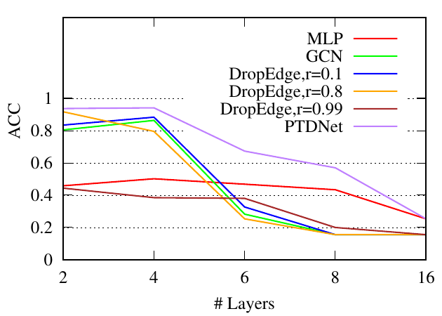
In this part, we experimentally demonstrate the effectiveness of PTDNet on alleviating the over-smoothing problem in GNN models with a very dense graph. We adjust the synthetic datasets used in the above section by adding more edges. With GCN as the backbone, we compare our PTDNet with DropEdge and the basic backbone. Since stacking multiple GNN also involves the overfitting problem, we include MLP as another baseline, which uses the identity matrix as the adjacency matrix. For DropEdge, we choose three dropedge rates, 0.1, 0.8, and 0.99. We range the number of GCN from 2 to 16 and show the results in Fig 8.
From the figure, we have the following observations. First, the performances of MLP w.r.t the number of layers show that the overfitting problem appears when 16 layers are stacked. Thus, for models with 8 or fewer layers, we can dismiss the overfitting problem and focus on the over-smoothing merely. Second, GCN models with 4 layers or more suffer from the over-smoothing problem, which makes the basic GCN model performance even worse than MLP. Third, DropEdge can only alleviate the over-smoothing problem to some degree due to its limitation on the testing phase. Last but not least, our PTDNet consistently outperforms all baselines. The reason is that our method is parameterized and can learn to drop edges during the training phase. The learned strategies can also be utilized in the testing phase to further reduce the effects of the over-smoothing.
|
Method | Cora | Citeseer | Pubmed | |||
| AUC | AP | AUC | AP | AUC | AP | |
| GCN(GAE) | 0.910 | 0.920 | 0.895 | 0.899 | 0.964 | 0.965 |
| DropEdge | 0.881 | 0.903 | 0.862 | 0.880 | 0.859 | 0.877 |
| NeuralSparse | 0.901 | 0.917 | 0.899 | 0.910 | 0.926 | 0.953 |
| PTDNet | 0.916 | 0.931 | 0.918 | 0.922 | 0.963 | 0.966 |
5.8 Link prediction. In this section, we apply our PTDNet to another downstream task, link prediction. We adopt the Cora, Citeseer, and Pubmed datasets and follow the same experimental settings in GAE, which applies GCN for link prediction [26]. PPI dataset is not used because it contains multiple graphs and not suitable for link prediction. Specifically, we randomly remove 10% and 5% edges for positive samples in the testing and validation sets. The left edges and all node features are used for training. We include the same number of negative samples as positive edges by randomly sampling unconnected nodes in validation and testing sets. We adopt area under the ROC curve, denoted by AUC, and average precision, denoted by AP, scores to evaluate their ability to correctly predict the removed edges. GCN is used as the backbone. We compare our PTDNet with the basic GCN, DropEdge and NeuralSparse. Performances are shown in Table 6. The table shows that our PTDNet can also improve the accuracy performance of link prediction. The denoising networks in PTDNet are optimized by the downstream task loss and can remove task-irrelevant edges. On the other hand, the performance between DropEdge and the original backbone shows that DropEdge is suitable for the link prediction task.
In this paper, we propose a Parameterized Topological Denoising Network (PTDNet) to filter out task-specific noisy edges to enhance the robustness and generalization power of GNNs. We directly limit the number of edges in the input graph with parameterized networks. To further improve the generalization capacity, we introduce the nuclear norm regularization to impose the low-rank constraint on the resulting sparsified graphs. PTDNet is compatible with various GNN models, such as GCN, GraphSage, and GAT to improve performance on various tasks. Our experiments demonstrate the effectiveness of PTDNet on both synthetic and benchmark datasets.
ACKNOWLEDGMENTS This project was partially supported by NSF projects IIS-1707548 and CBET-1638320.
[1] Raman Arora and Jalaj Upadhyay. 2019. On Differentially Private Graph Sparsification and Applications. In NeurIPS. 13378–13389.
[2] András A Benczúr and David R Karger. 1996. Approximating st Minimum Cuts in Õ (n2) Time.. In STOC, Vol. 96. Citeseer, 47–55.
[3] Yoshua Bengio, Nicholas Léonard, and Aaron Courville. 2013. Estimating or propagating gradients through stochastic neurons for conditional computation. arXiv preprint arXiv:1308.3432 (2013).
[4] Joan Bruna, Wojciech Zaremba, Arthur Szlam, and Yann LeCun. 2013. Spectral networks and locally connected networks on graphs. arXiv preprint arXiv:1312.6203 (2013).
[5] Andrew Carlson, Justin Betteridge, Bryan Kisiel, Burr Settles, Estevam R Hruschka, and Tom M Mitchell. 2010. Toward an architecture for never-ending language learning. In AAAI.
[6] Jie Chen, Tengfei Ma, and Cao Xiao. 2018. Fastgcn: fast learning with graph convolutional networks via importance sampling. arXiv preprint arXiv:1801.10247 (2018).
[7] L Paul Chew. 1989. There are planar graphs almost as good as the complete graph. J. Comput. System Sci. 39, 2 (1989), 205–219.
[8] JJ David. 1995. Algorithms for analysis and design of robust controllers. (1995).
[9] Michaël Defferrard, Xavier Bresson, and Pierre Vandergheynst. 2016. Convolutional neural networks on graphs with fast localized spectral filtering. In NIPS. 3844–3852.
[10] Talya Eden, Shweta Jain, Ali Pinar, Dana Ron, and C Seshadhri. 2018. Provable and practical approximations for the degree distribution using sublinear graph samples. In WWW. 449–458.
[11] Negin Entezari, Saba Al-Sayouri, Amirali Darvishzadeh, and Evangelos Papalexakis. 2020. All You Need is Low (Rank): Defending Against Adversarial Attacks on Graphs. In WSDM. ACM.
[12] Ky Fan. 1951. Maximum properties and inequalities for the eigenvalues of completely continuous operators. PNAS 37, 11 (1951), 760.
[13] Santo Fortunato. 2009. Community detection in graphs. CoRR abs/0906.0612 (2009).
[14] Shmuel Friedland and Lek-Heng Lim. 2018. Nuclear norm of higher-order tensors. Math. Comp. 87, 311 (2018), 1255–1281.
[15] Federico Girosi. 1998. An Equivalence Between Sparse Approximation And Support Vector Machines. Neural Computation 10, 6 (1998), 1455–1480.
[16] Marco Gori, Gabriele Monfardini, and Franco Scarselli. 2005. A new model for learning in graph domains. In IJCNN, Vol. 2. IEEE, 729–734.
[17] Will Hamilton, Zhitao Ying, and Jure Leskovec. 2017. Inductive representation learning on large graphs. In NIPS. 1024–1034.
[18] Gecia Bravo Hermsdorff and Lee M Gunderson. 2019. A Unifying Framework for Spectrum-Preserving Graph Sparsification and Coarsening. arXiv preprint arXiv:1902.09702 (2019).
[19] Yifan Hou, Jian Zhang, James Cheng, Kaili Ma, Richard T. B. Ma, Hongzhi Chen, and Ming-Chang Yang. 2020. Measuring and Improving the Use of Graph Information in Graph Neural Networks. In ICLR.
[20] Wenbing Huang, Tong Zhang, Yu Rong, and Junzhou Huang. 2018. Adaptive sampling towards fast graph representation learning. In NeurIPS. 4558–4567.
[21] Catalin Ionescu, Orestis Vantzos, and Cristian Sminchisescu. 2015. Matrix backpropagation for deep networks with structured layers. In ICCV. 2965–2973.
[22] Eric Jang, Shixiang Gu, and Ben Poole. 2016. Categorical reparameterization with gumbel-softmax. arXiv preprint arXiv:1611.01144 (2016).
[23] Wei Jin, Yao Ma, Xiaorui Liu, Xianfeng Tang, Suhang Wang, and Jiliang Tang. 2020. Graph Structure Learning for Robust Graph Neural Networks. arXiv preprint arXiv:2005.10203 (2020).
[24] Taiju Kanada, Masaki Onuki, and Yuichi Tanaka. 2018. Low-rank Sparse Decomposition of Graph Adjacency Matrices for Extracting Clean Clusters. In APSIPA ASC. IEEE, 1153–1159.
[25] Thomas N Kipf and Max Welling. 2016. Semi-supervised classification with graph convolutional networks. arXiv preprint arXiv:1609.02907 (2016).
[26] Thomas N Kipf and Max Welling. 2016. Variational graph auto-encoders. arXiv preprint arXiv:1611.07308 (2016).
[27] Qimai Li, Zhichao Han, and Xiao-Ming Wu. 2018. Deeper insights into graph convolutional networks for semi-supervised learning. In AAAI.
[28] Ruoyu Li, Sheng Wang, Feiyun Zhu, and Junzhou Huang. 2018. Adaptive graph convolutional neural networks. In AAAI.
[29] Christos Louizos, Max Welling, and Diederik P Kingma. 2017. Learning Sparse Neural Networks through 𝐿 0 Regularization. arXiv preprint arXiv:1712.01312 (2017).
[30] Andreas Loukas. 2020. What graph neural networks cannot learn: depth vs width. In ICLR.
[31] Jianxin Ma, Peng Cui, Kun Kuang, Xin Wang, and Wenwu Zhu. 2019. Disentangled Graph Convolutional Networks. In ICML. 4212–4221.
[32] Chris J Maddison, Andriy Mnih, and Yee Whye Teh. 2016. The concrete distribution: A continuous relaxation of discrete random variables. arXiv preprint arXiv:1611.00712 (2016).
[33] Andriy Mnih and Karol Gregor. 2014. Neural variational inference and learning in belief networks. arXiv preprint arXiv:1402.0030 (2014).
[34] Yuji Nakatsukasa and Nicholas J Higham. 2013. Stable and efficient spectral divide and conquer algorithms for the symmetric eigenvalue decomposition and the SVD. SIAM Journal on Scientific Computing 35, 3 (2013), A1325–A1349.
[35] Jingchao Ni, Shiyu Chang, Xiao Liu, Wei Cheng, Haifeng Chen, Dongkuan Xu, and Xiang Zhang. 2018. Co-regularized deep multi-network embedding. In WWW.
[36] James M Ortega. 1990. Numerical analysis: a second course. SIAM.
[37] Benjamin Recht, Maryam Fazel, and Pablo A Parrilo. 2010. Guaranteed minimum-rank solutions of linear matrix equations via nuclear norm minimization. SIAM review 52, 3 (2010), 471–501.
[38] Yu Rong, Wenbing Huang, Tingyang Xu, and Junzhou Huang. 2020. DropEdge: Towards Deep Graph Convolutional Networks on Node Classification. ICLR (2020).
[39] Franco Scarselli, Marco Gori, Ah Chung Tsoi, Markus Hagenbuchner, and Gabriele Monfardini. 2008. The graph neural network model. IEEE TNN 20, 1 (2008), 61–80.
[40] Prithviraj Sen, Galileo Namata, Mustafa Bilgic, Lise Getoor, Brian Galligher, and Tina Eliassi-Rad. 2008. Collective classification in network data. AI magazine 29, 3 (2008), 93–93.
[41] Kijung Shin, Amol Ghoting, Myunghwan Kim, and Hema Raghavan. 2019. Sweg: Lossless and lossy summarization of web-scale graphs. In WWW. ACM, 1679–1690.
[42] David C Van Essen, Stephen M Smith, Deanna M Barch, Timothy EJ Behrens, Essa Yacoub, Kamil Ugurbil, Wu-Minn HCP Consortium, et al. 2013. The WU-Minn human connectome project: an overview. Neuroimage (2013).
[43] Petar Veličković, Guillem Cucurull, Arantxa Casanova, Adriana Romero, Pietro Lio, and Yoshua Bengio. 2017. Graph attention networks. arXiv preprint arXiv:1710.10903 (2017).
[44] Chi-Jen Wang, Seokjoo Chae, Leonid A Bunimovich, and Benjamin Z Webb. 2017. Uncovering Hierarchical Structure in Social Networks using Isospectral Reductions. arXiv preprint arXiv:1801.03385 (2017).
[45] Lu Wang, Wenchao Yu, Wei Wang, Wei Cheng, Wei Zhang, Hongyuan Zha, Xiaofeng He, and Haifeng Chen. 2019. Learning Robust Representations with Graph Denoising Policy Network. IEEE ICDM (2019).
[46] Lichen Wang, Bo Zong, Qianqian Ma, Wei Cheng, Jingchao Ni, Wenchao Yu, Yanchi Liu, Dongjin Dong, and Haifeng Chen. 2020. Inductive and Unsupervised Representation Learning on Graph Structured Objects. In ICLR.
[47] Wei Wang, Zheng Dang, Yinlin Hu, Pascal Fua, and Mathieu Salzmann. 2019. Backpropagation-Friendly Eigendecomposition. In NeurIPS. 3156–3164.
[48] Ronald J Williams. 1992. Simple statistical gradient-following algorithms for connectionist reinforcement learning. Machine learning 8, 3-4 (1992), 229–256.
[49] Keyulu Xu, Weihua Hu, Jure Leskovec, and Stefanie Jegelka. 2018. How powerful are graph neural networks? arXiv preprint arXiv:1810.00826 (2018).
[50] F Xue and J Xin. 2020. Learning Sparse Neural Networks via l0 and l1 by a Relaxed Variable Splitting Method with Application to Multi-scale Curve Classification. In 6th World Congress on Global Optimization.
[51] Zhilin Yang, William W Cohen, and Ruslan Salakhutdinov. 2016. Revisiting semi-supervised learning with graph embeddings. arXiv preprint arXiv:1603.08861 (2016).
[52] Hanqing Zeng, Hongkuan Zhou, Ajitesh Srivastava, Rajgopal Kannan, and Viktor Prasanna. 2020. GraphSAINT: Graph Sampling Based Inductive Learning Method. In ICLR.
[53] Kai Zhang, Yaokang Zhu, Jun Wang, and Jie Zhang. 2020. Adaptive Structural Fingerprints For Graph Attention Networks. ICLR (2020).
[54] Ziwei Zhang, Peng Cui, and Wenwu Zhu. 2018. Deep learning on graphs: A survey. arXiv preprint arXiv:1812.04202 (2018).
[55] Lingxiao Zhao and Leman Akoglu. 2019. PairNorm: Tackling Oversmoothing in GNNs. arXiv preprint arXiv:1909.12223 (2019).
[56] Cheng Zheng, Bo Zong, Wei Cheng, Dongjin Song, Jingchao Ni, Wenchao Yu, Haifeng Chen, and Wei Wang. 2020. Robust Graph Representation Learning via Neural Sparsification. In ICML.
[57] Jie Zhou, Ganqu Cui, Zhengyan Zhang, Cheng Yang, Zhiyuan Liu, Lifeng Wang, Changcheng Li, and Maosong Sun. 2018. Graph neural networks: A review of methods and applications. arXiv preprint arXiv:1812.08434 (2018).
![∑︁𝐿 𝐿∑︁ ∑︁
||Z𝑙||0 = I[𝑧𝑙𝑢,𝑣 ≠ 0],
𝑙=1 𝑙=1(𝑢,𝑣)∈E](main0x.png)
![[ ]
∂𝑓--∂𝑔-
∇α𝑙𝑢,𝑣Eϵ1,...,ϵ𝐿𝑓({𝑔,X})= ∇α𝑙𝑢,𝑣Eϵ1,...,ϵ𝐿 ∂𝑔 ∂α𝑙𝑢,𝑣 .](main4x.png)