¨ Flow Network:
Given a directed graph G(V,E), and a function w: E(G) à R+.
We say w(e) is the edgecapacity of the edge e. We can suppose w(e)>0,
Otherwise we can remove the edge e from the graph.
¨ Source and Sink:
(a) capacity constraint: 0 £ f(e) £ c(e) for each edge e.
¨ Remark:
We have å f(s,u) = å f(u,t).
¨ Flow value:
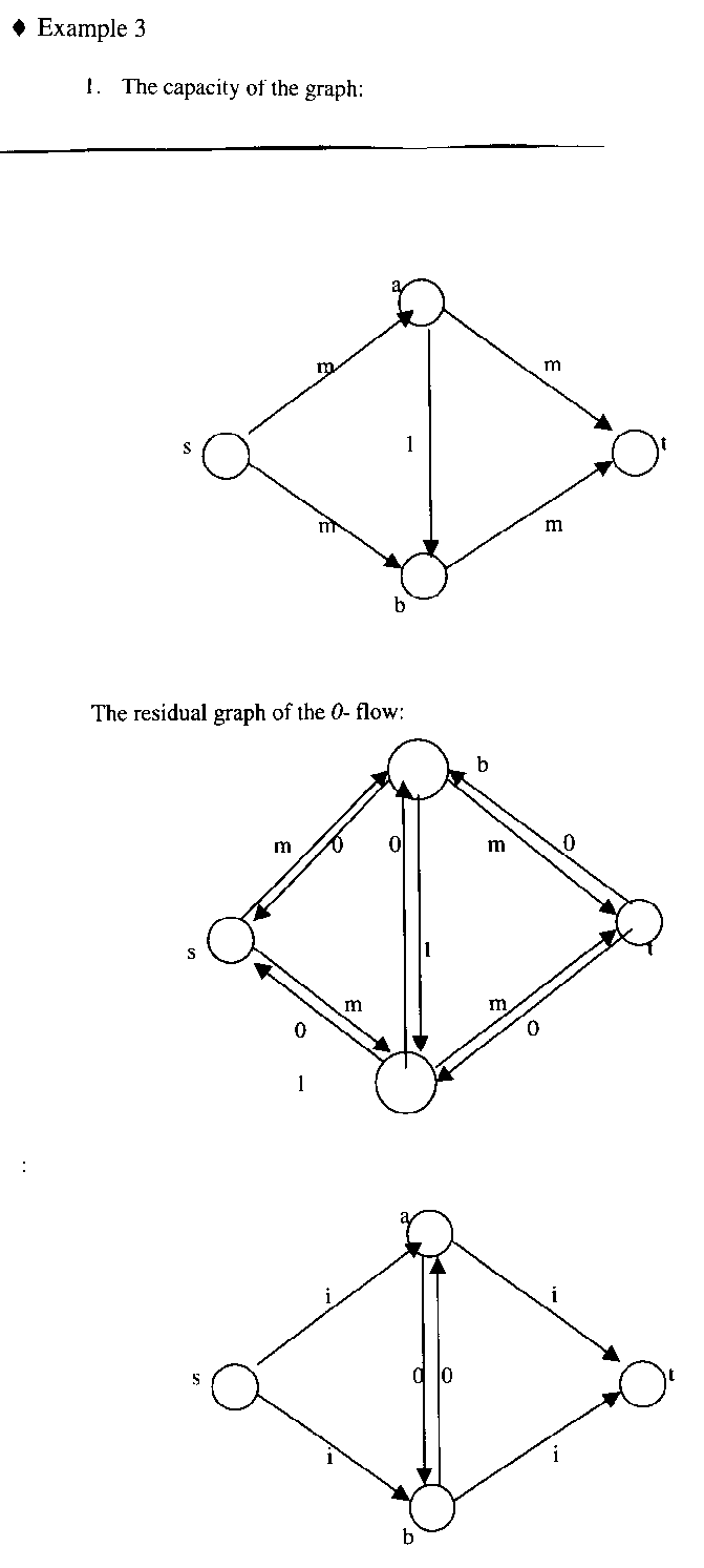
This flow has value 8.
¨ The residual network Gf for a flow f.
If (a,b) Î E(Gf) was originally orientated that direction in G, then
v(a,b):= w(a,b)-f(a,b), and v(b,a):=f(a,b). Note, that if (a,b) and (b,a) were both edges of G, then in Gf there are two (a,b) and two (b,a) edges.
If there is a path P = (s, a1), (a1, a2), {a2, a3), . . . , (al, t), and c>0 is the minimum weight of these edges in the residual graph, then do the following changes on the weights:
f?(s, a1):= f(s, a1) + c; ?. f?(al, t).
For each edge (a, b) of the path gives the following change of the weigtht on the residual graph:
v(a, b):= v(a, b) -c; v(b, a):= v(b, a) + c.
This method stops, if there is know path in the residual graph from s to t, with positive weigth on each edge.
The Ford- Fulkerson- Method (G, c, s, t)
¨ Correctness
The value of the flow is always increases, because we
have only outgoing edges from s. If we have no more augmenting path, then
it is the case, that there exists a cut with fully-flowed edges from s
to t, and by the max-flow= min-cut theorem we reached a maximal flow. For
more details see the book.
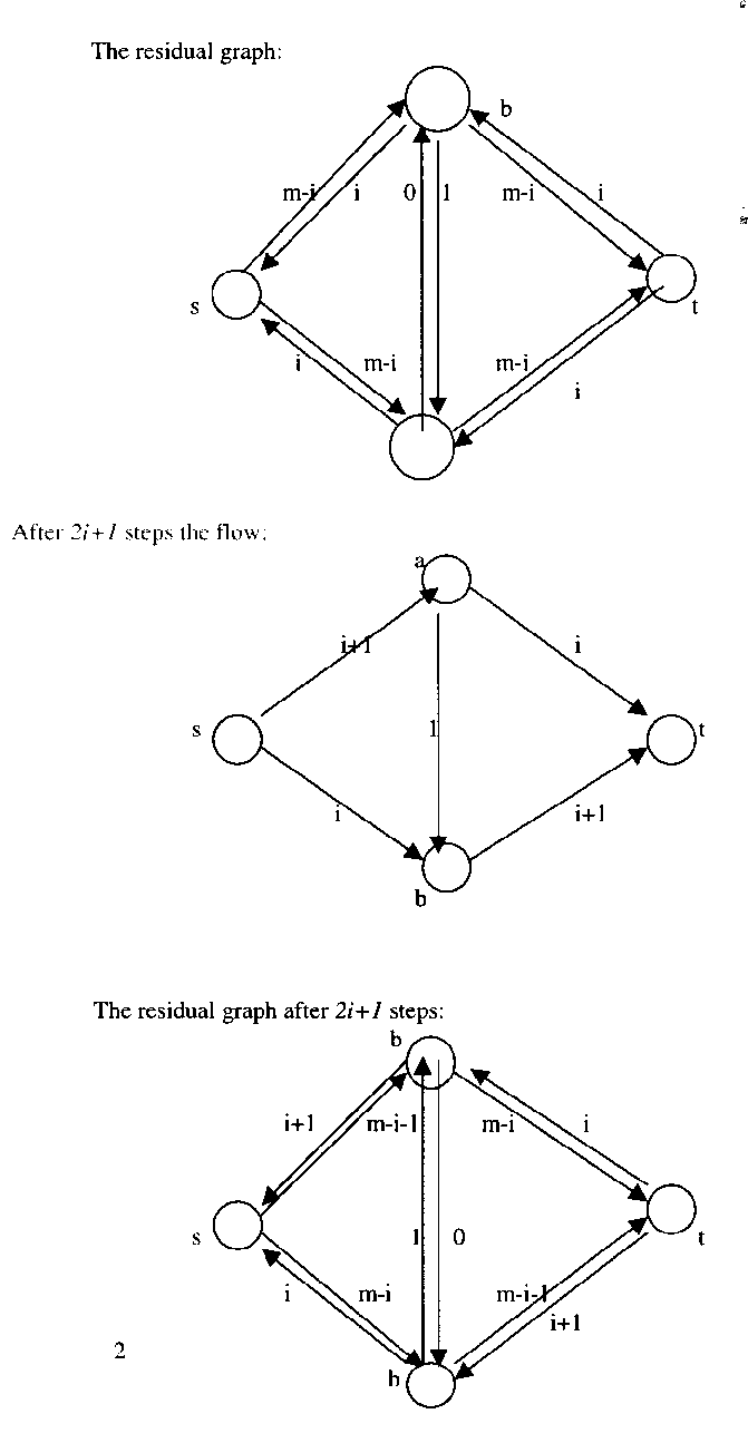
After 2i steps we have the following flow state and the following residual state:
So the time complexity 2m.
Easy to see, if we rather choose paths sat and sbt, then
two steps are enough.