algorithm

12/2: The difficult problems in algorithm programming

Noted by Zhijun Lu

1). Exhaustive Algorithm:

Some problems involve searching through a vast number of potential solutions to find an answer, and simply don't seem to be amenable to solution by efficient algorithm. For example, TSP problem is difficult because there seems to be no way to avoid having to check the length of a very large number of possible tours. Checking each and every tour is exhaustive search: first we'll see how that is done. Then we'll see how to modify that procedure to greatly reduce the number of possibilities checked by trying to discover incorrect decisions as early as possible.

a. Permutation Generation problem.

Suppose we have a set of number:

[1, 2, 3, …, n]

there are n! permutation

length of input = logN

length of output: = O(nn!)=exponential in logN

Permutation Algorithm

int id=-1
int N=4

Visit (int)
{
     int t;
     val[k]=++id;
     if (id==N) writeperm();
     for (t=1;t<=N;t++)
             if (val[t]==0)
               visit (t);
     id--;
    val[k]=0;
}

main()
{
    for (int I=1; I<=N; I++)
    val[I]=0;
    visit(0);
}

id = number of items in permutation that have been computed.
N=the number of each element in number set.

The result is as follows:

1234     2314
1243     2413
1324     3214
1423     4213
1342     3412
1432     4312
2134     2341
2143     2431
3124     3241
4123     4231
3142     3421
4132     4321

b. Exhaustive Search in Graphs

Algorithm:

Visit(int k)
{
     int t;
    // id is current length of path
    val[k] = ++id;
    for (t=1; t<=N; t++)
        if (Adj[k,t])
            if (val[t]==0) visit (t);
    id--;
    val[k] = 0;
}

This algorithm searches all possible paths. Similar depth search but waste a lot of time.

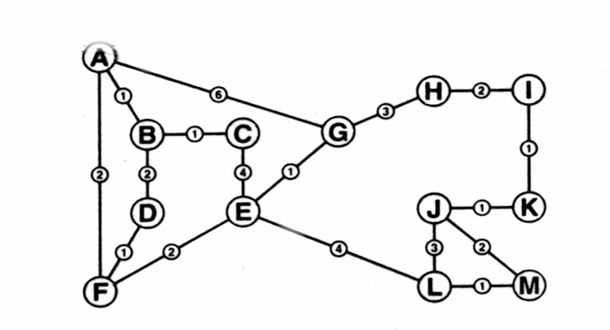
For example:
f1.jpg (44237 bytes)

Figure 1

This algorithm can change this graph into a tree as follows:

f2.jpg (124092 bytes)

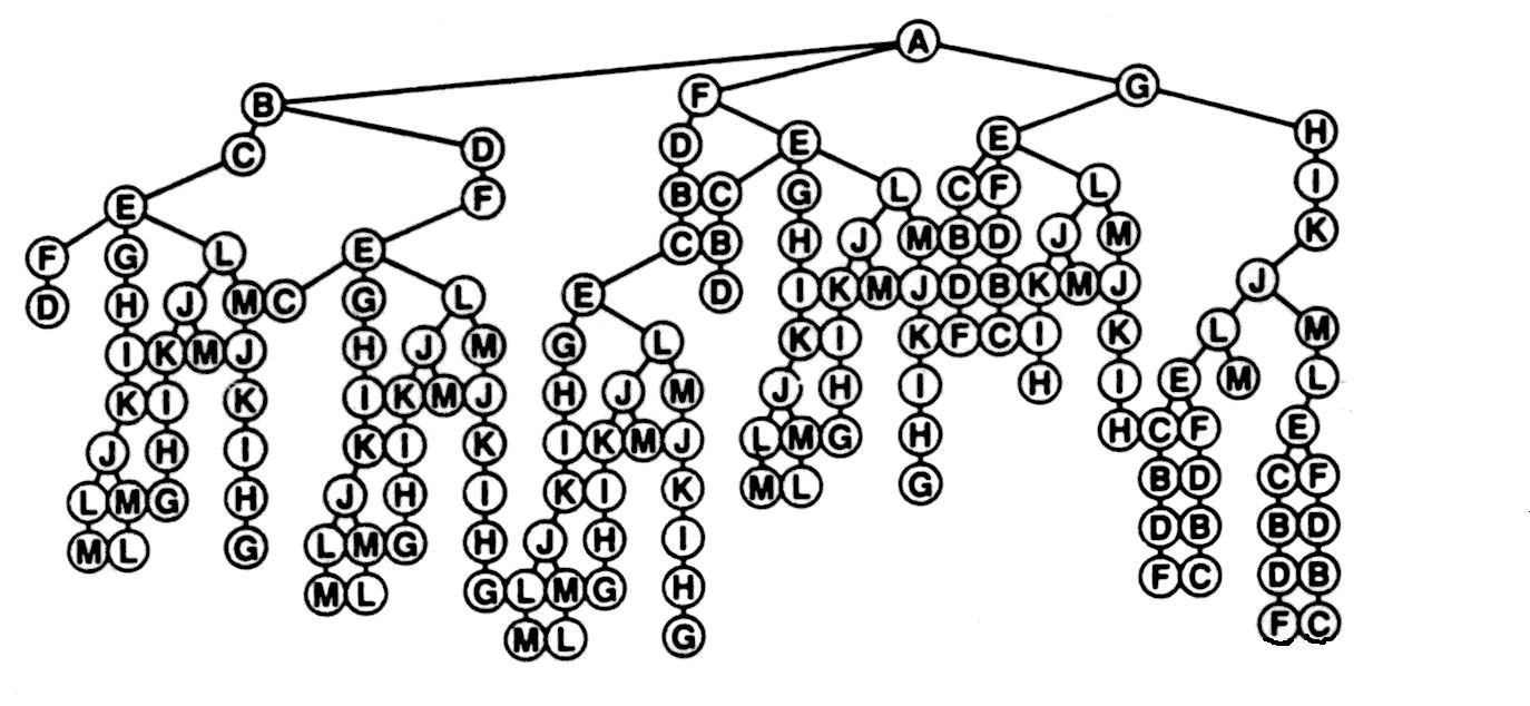
Figure 2

There are two possible ways to prune the tree:

Backtracking: solving a problem by systematically generating all possible solutions.

1. insisting that three particular nodes appear in a particular order. For example, if we insist that node C appear after node A but before node B, then we don't have to call visit for node B unless node C is already on the path, then we cut off the node avoiding searching the whole tree. This leads to the drastically smaller tree shown following figure 3.

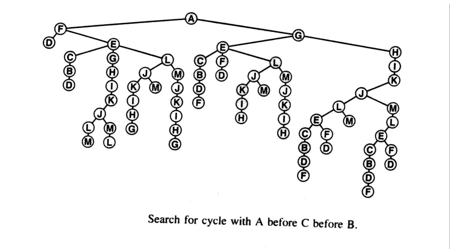
Figure 3

This technology can't be used when we can't know in advance whether a path will lead to a cycle or not.

Some paths might divide the graph in such a way that the unmarked aren't connected. For example, there can't be any simple path starting with AFE in Figure 1, since the path separates B, C, and D from the rest of the graph. Also a simple path storting wiht AGE sepatates B, C, D & F frp, tje rest of the graph. Following figure shows the search tree that results when this rule is applied to the tree of figure 3. The resulting figure is shown below in figure 4.

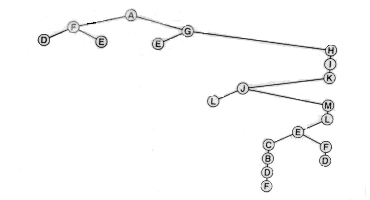f4.jpg (31773 bytes) Figure 4

Branch & Bound: calculate the bounds on partial solutions in order to limit the number of full solutions needing to be examined. for example, we can get a much better bound on the counts of any full path which starts with the partial path made up of the marked nodes by adding the cost of the minimum spanning tree of the unmarked nodes.

2. Linear Programming:
Linear programming helps solve optimization problems. If all of the equations or inequalitites involved can be expressed as linear combinations of the variables, we have the special case that we're considering called linear programming.

Considering the following:

You have a choice of n food items. There are m possible nutrients in each food item. Given:

a_ij = amount of i-th nutrient in the j-th food item
r_i= yearly requirement of i-th nutrient
c_j= unit cost of i-th food item
Design a yearly diet so that cost is minimized.

If we let x_j = yearly consumption of the j-th food item, then the problem can be redefined as follows:

Min c₁x₁ + c₂x₂ +…+ c_nx_n subject to:

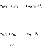
The above constraints can be written compactly in matrix form as where A is an , when A is an nxn matrix with enties [a_ij] .
Linear Programming can be solved in polynomial time.

3. Shortest st-Path Problem:
We show below that the shortest st-Path Problem can be written as a LP problem.
Let D be an incidence matrix such that if e_j=(i, k), then D[i, j]=+1, D[k,j]=-1, and all other entries on column j are 0. Note that the rows of D correspond to vertices. We will assume that the first two rows correspond to vertices s and t. Let the weight (or length) of edge e_jbe c_j.

Then the problem can be redefined as follows:

Min c₁x₁ + c₂x₂ +…+ c_nx_ns.t.
This problem is equal to find a solution to linear equation: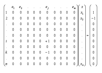