1. they run in polynomial time

2. they produce solutions close to the optimal solutions

Approximation algorithms are useful to give approximate solutions to NP hard problems. However, they can also be used to give approximate solutions to problems that run in polynomial time, in this case they are useful to give fast approximations.

1. EUCLIDEAN TSP

Algorithm 1: Greedy algorithm (2-approximation)

Always produces a TSP path that is at most twice as long as the optimal TSP path

Algorithm 2: Christofides algorithm (3/2 approximation)

2) VERTEX COVER PROBLEM

Algorithm 1: Greedy algorithm 2-approximation

Algorithm 2: Vertex greedy algorithm

Coming out with a heuristics is quite simple. However, proving any property of the heuristics is quite difficult.

Next, a counterexample shows that algorithm 2 to solve the vertex cover problem is worse than algorithm 1.

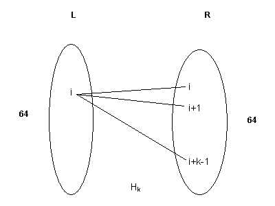
Basic device

Figure 1. Basic device, to build the graph. Each piece has 64 vertices and each vertex has degree k.

H_k is a bipartite graph such that each part of the graph has 64 vertices, and vertex i from L is connected to the vertices i, i+1, …, i+k-1, of R as shown in the figure 1. The values i+j are computed mod 64, i.e., if i+j is greater than 64 then the indices wrap around starting from 1, again.

Figure 2. Graph used as a counterexample to show that the vertex greedy algorithm is worse than the 2-approximation algorithm. The numbers at the side of every piece, represent the degrees of each vertex. Only the edges for the first left-hand piece are shown. The other left-hand pieces have the same amount of edges as the first one.

Each piece has 64 vertices (just as described above). Only the edges for the first piece are shown, the other two pieces have the same amount of edges to each of the other pieces at the right-hand side.

As is shown in the figure 2, each vertex at the upper left piece has 64 (1+1+2+4+8+16+32) edges, i.e., all its vertices have degree 64. Therefore, each vertex in the pieces at the left-hand side has degree 64.

On the other hand, each vertex of the upper right piece has three edges (one to each left-hand piece), and the same applies to the second upper right-hand piece. In other words, each vertex belonging to any of these two pieces has degree 3.

Similarly, each vertex in the third right-hand piece has degree 6 (two edges to each left–hand piece). The vertices in the fourth, fifth, sixth and seventh right-hand pieces have degree 12, 24, 48 and 96, respectively (4x3, 8x3, 16x3 and 32x3, respectively).

The degrees of each vertex in every piece are shown at the side of each piece in the figure 2.

The optimal vertex cover is made up of the set of vertices in the three pieces at the left-hand side. This set has 3x64 vertices.

The vertex greedy algorithm first picks every vertex of degree 96 (maximum degree). After picking these 64 vertices, each vertex at the left hand-side pieces have degree 32, since 32 edges incident on each of them have already been "covered". Therefore, in the second stage, the algorithm picks the 64 vertices of degree 48. After choosing all the vertices of degree 48, each vertex at the left-hand side has degree 16, because the other 16 edges have already been covered.

In the third step, the 64 vertices of degree 24 are chosen, because they have the current maximum degree. After this stage, each vertex of the left-hand pieces has degree 8 (8 edges have been removed per vertex).

The algorithm continues picking up the remaining vertices on the right hand side, from the bottom to the top, the ones with degree 12, 6, 3 and 3, respectively.

Therefore, the vertex greedy algorithm picks all the vertices from the pieces at the right-hand side, that is, 7x64 vertices.

The approximation given by the vertex greedy algorithm, in this case, is seven times the size of the optimal solution.

|VC|_greedy = (7/3)x |VC|_opt

Some problems are easier to approximate than others, and NP-hard problems can be classified according to their approximability.

Good approximation algorithms guarantee an approximation of the optimal solution up to a constant factor.

Since any NP hard problem can be reduced to any other NP hard problem, one might think that this could help to develop good approximation algorithms for all NP-hard problems. However, this is not true as can be seen in the next example.

Let us consider the vertex-cover problem, clique problem and the independent set problem, which are very closely related.

Consider the problem of finding the largest independent set or a clique in a given graph G.

If G has a clique of size greater than or equal to k then G (G complement) has a vertex cover of size less than or equal to n-k.

If G has an independent set of size greater than or equal to k then G has a vertex cover of size less than or equal to n-k.

How to use the approximation algorithm to find a vertex cover in order to produce an approximation algorithm to find an independent set?

Consider the following algorithm.

Given a graph G, compute a vertex cover using the greedy approximation algorithm and output the rest as an independent set.

However, the 2-approximation algorithm to the vertex cover problem cannot be used directly to give a good approximation to the independent set problem. For instance, let us assume that the optimal solution to the vertex problem has 49 vertices, and the maximum independent set has 51 vertices. Then the greedy approximation algorithm guarantees a solution of up to 98 vertices. Therefore, by looking at the complement graph G, this algorithm guarantees a independent set of at most size 2, which is a very bad approximation, since the optimal solution has 51 vertices.

This example shows that reductions do not help in developing approximation algorithms.

Good approximation algorithms give an approximation up to a constant factor. Examples of good approximation algorithms are the Euclidean version of the TSP problem, and the vertex cover problem.

On the other hand, there are some problems for which no constant factor approximation is possible, for instance, the clique, independent set and TSP (not Euclidean version) problems.

Another kind of approximation algorithms are considered better than good: in this case, an approximation scheme exists, i.e., the algorithm guarantees solutions within any arbitrary factor, if you can afford spending more time. However, there are some problems for which it can be proved that no approximation scheme exists.

Example: 3-COLORING PROBLEM

Instance: a graph (V, E)

Question: Can V be "legally" colored with 3 colors; "legally" means that no two adjacent node share the same color.

A c-approximation means that 3*c colors are used to color "legally" the graph

For example, c < 4/3 is impossible unless P=NP

No known algorithm can guarantee using fewer than colors even if it knows that 3 colors are sufficient.

Example: EDGE COLORING PROBLEM

Instance: a graph (V, E)

Question: Can E be "legally" colored with k colors; "legally" means that no two adjacent edges are the same color.

Vizing's theorem states that d or d+1 colors are enough to legally color E, with d the maximum degree of any vertex in the graph.

There is a polynomial time algorithm that colors with d+1 colors.

Example: 0-1 KNAPSACK PROBLEM

Instance: n items each with values v₁, v₂, ...,v_n, and weights w₁, w₂, ...,w_n, respectively. Let B be the weight bound.

Question: what is the number of copies of each item to be chosen such that their total weight is less than or equal to B, and the value is maximized.

In mathematical terms, find x₁, x₂, ..., x_n such that

x₁*v₁+ x₂*v₂+ ...+ x_n*v_n is maximum

and

x₁*w₁+ x₂* w ₂+ ...+ x_n* w _n £ B

solution: (using dynamic programming)

M[i,j] : maximum value that can be packed with weight bound j using items from {1, 2, 3, ..., i}

The matrix is filled in row by row, from the top to the bottom.

M[i,j] = max {M[i-1, j], M[i, j-w_i]+v_i}

Time complexity O(nB)